Income FAQ

1. Why is the Average Household Income in my Model Overview so High?

In IMPLAN, we base household income on the Bureau of Economic Analysis (BEA)’s “Personal Income” numbers controlled to current BEA National Income and Product Accounts (NIPA) for the nation. In contrast, per capita household income reported by the Bureau of the Census is “Money Income” based. Due to a number of data source differences, definitional differences, and variances in scope and purpose the numbers reported in these two data sources vary significantly. For more information about these differences please explore this article

2. Why are Oil & Gas extraction sector proprietors appearing in a study area that does not in reality contain oil wells?

This is due to how Proprietors are accounted for in the IMPLAN system. Unlike the place-of-work Wage and Salary data used by IMPLAN to account for employees, the Proprietor Employment data are place-of-residence based. That is, a well-owner who lives in NJ but whose well is in another state will show up in the BEA data (and subsequently, in the IMPLAN data) as a proprietor in O&G extraction sector in the NJ data set. That proprietor is then allocated a certain proportion of the U.S. O&G extraction output, since the output data are reported at the U.S. level only.

In addition, the BEA considers ownership by partnership a proprietor. Therefore, it is possible to have many partners in oil and gas in a county in which there is no oil and gas.

3. Why are there different definitions for GRP?

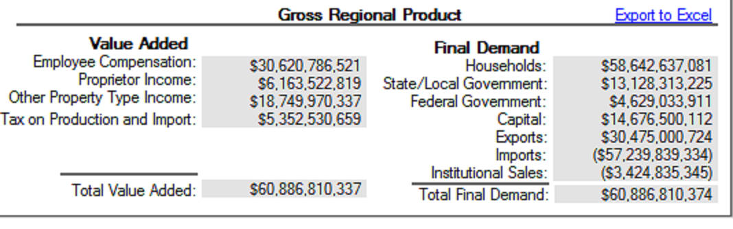
Gross Regional Product describes the wealth in a region and is a common measurement of economic stability and growth. GRP can be measured on an expenditure basis (Final Demand) or on an income basis (Value Added); thus the Model Overview screen provides a breakdown of GRP looking at both measurements.

  • Final Demand describes the value of goods & services produced and sold to final users during the calendar year. These final users would include governments, households, exports (net), and investments (Capital).
  • Value Added describes how income is distributed to these same Institutions or final users.

Looking at the Model Overview

Viewing the Model Overview we can see that just because the method of measurement differs, since both methods measure GRP, the resultant value is the same (some variance will occur after the first seven significant digits due to rounding).


pic1.png

Value Added Final Demand
Employee Compensation: The entire cost of employees including wages and salaries payroll taxes and benefits: sometimes referred to as fully-loaded wages or income. This value is a primary source for households and a source of monies for governments (in the form of payroll taxes) for final demand purchases. Households: Households make payments to industries for goods and services used for personal consumption (PCE) and to governments in the form of taxes, fees, fines, etc. This is the largest component of final demand and is derived from household income in the region as a result of Employment Compensation, Proprietor Income and Other Property Type Income payments to households, as well as governments and payments from other households. Thus payments from these Value Added categories provide the basis of household consumption in final demand.
Proprietor Income: Income for sole proprietors and partnerships that drive household income for final demand and tax payments via income taxes for governments. State & Local Governments: Public education purchases are for K-12 and higher education institutions. Non-education purchases are for all other state and local government administration activities including police protection and sanitation. Funds for these purchases result household income as well as corporate taxes captured from Employment Compensation (payroll taxes and income taxes), Proprietor Income (income taxes), Other Property Type Income (income taxes) and Taxes on Production & Imports (fees, fines, sales taxes, licenses, etc).
Other Property Income: Income derived from dividends, royalties, corporate profits, payments for rent, and interest income. Thus Other Property Type Income provides a source of income for households, business, and govenments. Federal Government: Federal defense includes spending by all agencies in the Department of Defense. Non-defense purchases are made to supply all other Federal government administrative functions. Federal Investment consists of all Federal government demand for capital goods. Funds for these purchases result fromhousehold income as well as corporate taxes captured from Employment Compensation (payroll taxes and income taxes), Proprietor Income (income taxes), Other Property Type Income (income taxes) and Taxes on Production & Imports (fees, fines, sales taxes, licenses, etc).
Taxes on Production & Imports: Sales and excise taxes, customs duties, property taxes, motor vehicle licenses, severance taxes, other taxes, and special assessments. Subsidies are netted out and thus can be negative for some industries in some years. Thus, this is primary source for income for governments for final demand. Capital: Household savings and private industry purchases of capital equipment and construction, driven by corporate profits captured in the Other Property Type Income component of Value Added.
  Exports: Goods and services produced within the geography of the Model sold to both domestic and foreign buyers. These exogenous purchases by industries and households in other regions provide income (Employment Compensation, Proprietor Income and Other Property Income) to local households and corporations and to governments as taxes (Taxes on Production & Imports, Other Property Income and payroll taxes).
  Imports: Purchases of goods and services by households, governments and industries from outside the region that represent a loss of income to the Model geography. Imports are wealth leaked to other regions.
  Institutional Sales: Sales of goods and services by Institutions.  These are subtracted from the other components of Final Demand.

In both cases the total wealth in the economic geography is identical. On the Value Added side we see how Industries contribute to that growth through production, and on the Final Demand side we view how consumption drives local industries to produce products for local demand.

Read More

Employment FAQ

 1. How is IMPLAN Employment defined? 

Employment data in IMPLAN follows the same definition as Bureau of Economic Analysis Regional Economic Accounts (BEA REA) and Bureau of Labor Statistics Census of Employment and Wages (BLS CEW) data, which is full-time/part-time annual average. Thus, 1 job lasting 12 months = 2 jobs lasting 6 months each = 3 jobs lasting 4 months each. A job can be either full-time or part-time.  Similarly, a job that lasts one quarter of the year would be 0.25 jobs.  Note that a person can hold more than one job, so the job count is not necessarily the same as the count of employed persons.

Thus, while IMPLAN employment adjusts for seasonality, it does not indicate the number of hours worked per day. Thus, if you are using a full-time equivalent (FTE) value to add into IMPLAN results or as the proxy for an Event you will want to convert the FTE value to IMPLAN jobs prior to using it with IMPLAN. Conversely, if you need to report FTEs you will want to convert the IMPLAN jobs to reflect those. FTE and wage and salary to Employment Compensation conversions can be found in our Downloads section. Just choose the sectoring scheme appropriate for you data and download the related file. Whichever way you are converting, please keep in mind that FTE jobs are always fewer in number than the equivalent Part-time/Full time jobs.

The BEA calculates the number of FTE employees in each industry as follows:
FTE employees = (total number of employees) * [(average weekly hours per employee for all employees) / (average weekly hours per employee on full-time schedules)]
As for their determination on the number of hours for defining “employees on full-time schedules”, the BEA uses BLS as a source and adopts their definition of full-time which is accounted for as anyone working 35 hours or more.

The output per worker relationships are based on the average annual job. So if a worker works 6 months, they have half the annual output and that worker will need to be entered as 0.5 jobs. To adjust the seasonal employment, take the job count times the number of months worked divided by 12. In equation form:
IMPLAN Jobs = Seasonal Jobs * [(months of seasonal job)/12]
Seasonal Jobs = IMPLAN Jobs / [(months of seasonal job)/12]

To keep in mind:

  1. If an industry is dominated by part-time workers this will be reflected in the earnings per worker.
  2. Employment itself is merely descriptive in the sense that it does not drive the Indirect or Indirect Effects.
  3. The Total Employment figure in the Model Overview screen represents full and part-time annual average including the self-employed, all federal, state, and local government employment and military employment (including overseas military).

2. Why does the Employment count in the Study Area Data differ from what is reported in other data sources? 

IMPLAN jobs include workers that are not accounted for by a number of other data sources. This often means that IMPLAN jobs are larger than many other sources report.

Learn more from our Knowledge Base:

Comparison of IMPLAN source data for Employment and Labor Income

Datasets used to create IMPLAN Employment data

Special Sectors for Employment data

Estimating non-disclosures when creating Employment and Labor Income databases

What if your reported Employment value is actually smaller than the reported value from another data source? This can happen because of BEA’s rules for redefinitions. Following these rules we redefine some reported Employment, income and production to other Sectors. If your IMPLAN Study Area Data shows less Employment than another report, feel free to post the region, data year and Sector on our community section and we can dig a little deeper to see if redefinitions are involved.

3. What are the differences between Employment Multipliers and Employment Effects? 

All Multiplier derivations are based off of Output. Knowing regional total Output and regional total Employment we can create Output per Worker relationships from which we can estimate the number of employees needed per million dollars of Output.

In the Employment Multiplier sheet, Direct, Indirect, and Induced are actual jobs/ million dollars of production.

The resulting Type I and Type SAM Multipliers are derived as follows:

Type 1 (Direct Employment + Indirect Employment/ Direct Employment)

Type SAM (Direct Employment + Indirect Employment+ Induced Employment/ Direct Employment)

4. How does IMPLAN verify the total number of jobs created for modeled Events? 

It is important to remember that IMPLAN jobs are not FTEs. Instead, IMPLAN follows the BEA job definitions, which include full-time, part-time, and seasonal jobs. Additionally, verification of the Direct Effect should be relatively easy based on the economic change defined. Generally speaking, we feel that, unless there are large numbers of jobs reported in the Indirect and Induced Effects, that these impacts are largely supported rather than created. This can be demonstrated by looking at the Detail Results of your impact and also by comparing the jobs associated to the impact to the current Employment in the impact Sectors. Unless the change of Employment in the Indirect and Induced Effects are significant in comparison to the current Employment in the Sector, we recommend considering it supported rather than created. In addition, many attempts have been made over the years to verify Indirect and Induced jobs, and this has proved very difficult to actually discern.

The “536 FTE & Employment Compensation Conversion Table” allows you to convert between IMPLAN jobs and FTEs or FTEs and IMPLAN jobs with simple rations for each Industry for the 536 Sectoring scheme. Using another year? Check out the Downloads section to find the Sectoring scheme you are working with and download its FTE and Employment Compensation conversion table.

5. The jobs associated to my short-term impact analysis seem too small. What went wrong? 

IMPLAN is an annual Model; therefore the Model will assume that the value being entered as Industry Sales represents production over a year’s time. Therefore the Employment estimates provided by the software represent annualized Employment values. When you shrink the quantity of production into a smaller time frame more jobs will be necessitated for the same level of production to occur. Unfortunately there is no ‘best’ way to adjust for this, and the analyst must use their personal knowledge of the region and Event to account for the changes they want to make to the Employment count. There is no preferred method because IMPLAN has a fixed Output per Worker ratio and therefore cannot adjust for the possibility that a single worker may be able to do more if there is sufficient demand for them to do so. It also cannot account for temporary shifts in workforce resulting from short-term events such as the movement of a part-time job to a full-time job for the period of increased production/demand. 

6. How should jobs associated to multi-year construction impacts be reported? 

We recommend that you divide the impact over the number of years of the project and report the average jobs per year.

For example, if a construction site generates 85 jobs across 3 years, then the report would state the supported jobs as 85/3 or 28 jobs per year. This is because the jobs on the construction site are not cumulative, in the same way that an employee working a job for 3 years is not viewed as 3 jobs.

We also recommend considering construction jobs as supported instead of created since construction jobs are typically site-to-site and the jobs on the site are constantly changing based on the state of the construction project.

7. If I have an operational impact that occurs year-over-year are the job impacts summative? 

Job impacts in year over year operational impacts should not be summed. 

Consider this scenario:

Blooms Garden Center opens in 2016 and creates 50 jobs. In 2017, there operations also support 50 jobs, but this does not mean that Blooms Garden Center supports 100 jobs. Instead it means that they support 50 annual jobs. Note also that the jobs are only called ‘created’ in the first year.

What if the company has incremental employment increases planned?

If Blooms Garden Center purposes that they will expand to add 20 jobs in 2018 then:

    • You could look at the impact of their adding 20 jobs in 2018 and the additional sales associated to that.
    • You could look at the effect of 70 jobs at Blooms Garden Center in 2018
    • The new year-over-year impact would be 70 supported jobs.

8. Why do the Government Employment & Payroll Sectors start with an *? 

These are specialty Sectors that represent just government payroll and Value Added. As such these Sectors have no Intermediate Expenditures associated to them and will generate no Indirect Effects. If you are looking to Model the effects of government spending in your region, we recommend you use the appropriate government spending pattern found at Activity Options>Import> Institutional Spending Pattern or a spending pattern from the SpendingPatternsNoPayroll_for_Programs_by_SLGovt. For IMPLAN Pro users, you may already have these spending patterns in you Activity Options> Import> From Another Model>IMPLAN User Data >Utilities if not you can download the library for your Sectoring scheme here. If you are in IMPLAN-Online you can request a spending pattern for your government Activity Type from the list of available spending pattern types and we can send it to you. 

The spending patterns found in your Activity Options menu are updated annually but are more generic in their description. Those found in the library are updated every 5 years but are more specific in their description of government activities.

Available spending patterns from the SpendingPatternsNoPayroll_for_Programs_by_SLGovt are:

Federal Govt operating budget expenditures national defense
Federal Govt gross investment national defense
Federal Govt operating budget expenditures nondefense
Federal Govt gross investment nondefense
State & Local Govt operating budget expenditures elementary and
State & Local Govt operating budget expenditures public educatio
State & Local Govt operating budget expenditures other education
State & Local Govt construction elementary and secondary public
State & Local Govt construction public educational facilities be
State & Local Govt invest other education and libraries
State & Local Govt operating budget expenditures hospitals and c
State & Local Govt operating budget expenditures public welfare
State & Local Govt operating budget expenditures sanitation
State & Local Govt construction hospitals and categorical health
State & Local Govt construction public welfare institutions and
State & Local Govt construction public sewerage systems
State & Local Govt construction sanitation
State & Local Govt operating budget expenditures police
State & Local Govt operating budget expenditures fire fighting o
State & Local Govt operating budget expenditures correctional in
State & Local Govt construction police
State & Local Govt construction fire fighting organizations and
State & Local Govt construction correctional institutions
State & Local Govt operating budget expenditures public highways
State & Local Govt operating budget expenditures natural and agr
State & Local Govt operating budget expenditures other general g
State & Local Govt construction public highways
State & Local Govt construction waterports and airports
State & Local Govt construction government-operated transit syst
State & Local Govt construction other commerce activities n.e.c.
State & Local Govt construction gas and electric utilities
State & Local Govt construction government-operated water supply
State & Local Govt construction redevelopment projects
State & Local Govt construction natural and agricultural resourc
State & Local Govt construction other general government activit

Learn more from our Knowledge Base:

Working with Government Institution Spending Patterns

Government Expenditures and Sales

Working with Military Bases

Electricity Generation + Distribution FAQ

We get a lot of questions on how the electricity generation and distribution data is handled in IMPLAN.  The following outlines the steps.

  • First, generation by sector is gathered in Megawatt-hours (MWH) from the US Energy Information Administration
  • Next, we obtain total revenue for all electricity from the US Energy Information Administration
  • With the value from #2 and the sum of total generation from #1, we calculate a revenue per MWH value, which we multiply against the generation by sector from #1 to get an estimate of revenue by sector.
  • We then split that revenue by sector into generation vs. distribution using the share of price between generators and distributors – http://www.eia.gov/electricity/annual/html/epa_02_04.html.
  • Finally, we split between private, federal, state, and local based on CEW data, which have enough detail for all generation types plus distribution.


RELATED TOPICS:

Methodology for Development of the 2017 Detailed Production Functions for IMPLAN’s Nine Electrical Power Sectors

Utility Purchases & Energy Rebates

Data FAQ

1. How often do I need to update my data?

In general, we leave this up to you. The multipliers are based on the structure of the economy of the year of the data. If you determine that the data year you have is an accurate representation of the current economy, then there is no need to update and purchase a more recent data year.

Here are some situations when IMPLAN Does recommend updating your data:

  • An obvious change in the local structure of the economy. Not all changes in local economies will be as obvious as New Orleans before and after Hurricane Katrina struck. In many cases, it may be growth of a subsector or even the introduction of new industries. The multipliers are based on the structure of the economy, whether an industry exists and the relationships of the demand and supply of commodities. Due to increases in foreign imports, Output Multipliers typically decrease in size somewhat over time. Likewise, as productivity increase, this also indicates decreased employment needs per dollar of output.
  • When a BEA Benchmark is released, IMPLAN follows suit and introduces those new underlying sets of industry production functions. The economy and technology are constantly changing. When new Benchmarks are introduced, new industries are likely introduced as well. If you wish to keep current with the BEA benchmark when reporting your analysis, a recent purchase of that data region is necessary to maintain consistency.
  • Scrutiny of the project using the data. The more exposure an analysis has to the public, particularly a controversial proposal with an opposing side, the more politically important it is to use “the latest data”.

Please feel free to post any additional questions to our Community.

2. How does IMPLAN handle Employment and other factors (e.g., Output, Income, etc.) in the Study Area Data when the Industry or interest, such as a casino hotel, performs several functions?

By definition, Employment in IMPLAN is a head count and not an FTE equivalent. For more information about the definition of IMPLAN Employment, please see our glossary.

While IMPLAN employment and income figures generally start off larger than CEW figures due to the addition of proprietors and proprietor income, a proportion of some sectors’ activity (employment, output, income, etc.) is later reclassified into other sectors. This reclassification process follows the BEA “redefinition” practice and is designed to reassign products from producing industries in which they are secondary products to the industries where those products are primary. Consider a popular hotel on the Las Vegas Strip. Such a hotel typically boasts a casino, restaurant, gift shop, and concert stage and would not be very well represented by the production function, income per worker ratio, output per worker ratio, and other factors of the hotel and motel sector. Therefore, IMPLAN utilizes the national redefinition table from the BEA to “redefine” certain small portions of the industry’s activity to other appropriate sectors such as Gambling (495), Restaurants (503), various Retail, and Performing Arts (488).

3. Does changing the size of Industry affect the Multipliers?

It seems counterintuitive, but a Sector’s Multiplier does not depend on the Sector’s overall size. Instead, what affects the Multiplier is the underlying relationships used in the creation of the Multiplier (specifically, Labor Income per $1 Output and Intermediate Expenditures per $1 of Output) of that Industry. When you run an impact analysis, it does not matter what the initial size of the Industry is – so long as those Industry relationships are what they should be.

4. Why is my impact smaller at the state level than at the county level?

It is true that generally a larger region has less leakages due to imports and therefore is typically a larger impact. However, depending on the industry mix of the county and the region(s) you are comparing it to, the RPCs for what is regionally available in a smaller region can exceed that of a larger region. This typically occurs when the primary region is a key producer of the commodities being examined in the study (or in generally represents the largest functional economy in the region) and thus a larger area increases demand at a faster rate than it provides additional supply, thus reducing the RPC values. However, a key problem also is that while it may seem like you are comparing like regions, because of the nature of Industry aggregation, you are comparing two distinct Multiplier identities. There are two methods for solving this, MRIO and Customization.

For more on this topic, visit our Knowledge Base article “Size of Your Impact – Small vs. Large Study Region“.

5. Why is my Value Added value negative?

Negative values in Value Added are a common source of confusion. Value Added = Employee Compensation + Proprietor Income + Other Property Type Income + Taxes On Production & Imports. PI, OPI, and TOPI can all be negative and if any one or a set of these sum to a more negative than the positive values (i.e., if the negative components are greater in magnitude than the positive components, then you will end up with negative VA). For example in the 2011 US Model Sectors 348 and 349 (both of which produce commodity 3348) have negative OPI. Negative OPI just means that the industry lost money that year (costs were greater than revenues). You can check to see exactly what is the circumstance in your regional industry by going to the Explore> Study Area Data and looking at the View By: Industry Detail sheet to see the breakdown of Value Added and to view which factor is causing the Value Added to be negative. If the factors involved are Other Property Type Income or Taxes on Production & Imports these do not impact the Indirect and Induced results as both of these factors are treated as leakage.

6. What is the difference between Impact vs. Contribution Analysis?

Two general categories of studies using IMPLAN have emerged over the years:  

Impact Analysis is the more common of the two. This type of study examines the economic impacts of an event or change to the economy (e.g., the opening of a new business). These studies address the general question: What are the marginal impacts of the project?

Contribution Analysis is becoming increasingly more common and concerns the role, importance, or contribution of an existing business, project, or industry. These studies address the general question: What is the contribution of the project to the overall economy of the area? 

Contribution Analysis in IMPLAN
Contribution Analysis using IMPLAN Online
Contribution Analysis using IMPLAN Pro

7. Why are Multipliers from OECD Countries low and how are they calculated?

The difference in Multipliers you will see when running an analysis using OECD data is not in how they are calculated but in the extent of the Indirect and Induced effects within a region for a Sector. The Direct Multipliers are always one. If the Sector in the region imports more of its inputs and if more households make purchases outside the region then the Multipliers will be smaller. In addition, – Germany is a smaller country than the U.S. and would be expected to have smaller RPC’s for many commodities.

Another reason is that in the OECD data, (PI) Proprietor Income is not separated out from OPI (Other Property Income); rather, there is just a single GOS (Gross Operating Surplus) category and it is not endogenized (i.e., it is treated like a leakage like OPI is in the standard IMPLAN data and does not generate Induced effects). Thus, Multipliers for all OECD countries will be somewhat lower due to this (including the U.S. OECD Model). If you are comparing to a ‘normal’ (i.e., 536-sector) U.S. Model, the Multipliers are not comparable because the U.S. Model spends PI, which increases the Induced effects and thus the Type SAM Multipliers.

Learn more about how the OECD data is created, what information it contains, and the possibilities and requirements for ordering custom created city, state, or provincial level international data sets.

Construction FAQ

What Value Is Entered for Industry Sales of a Construction Impact?

For the new construction sectors, output is the total value of the structures being built within the region, but does not include items that are not integral to the structure itself. So the Industry Sales value includes the total construction budget (payroll + non-payroll) plus any profits and indirect business taxes (i.e., taxes on production) paid by the construction firm.
This forum discussion addresses the difference between output and budget.

How Do I See What Soft Costs are Included in the Construction Sectors?
You can view the current spending pattern of the construction sector you are working with in the Regions>Region Overview>Social Accounts>Balance Sheets>Industry Balance Sheet>Commodity Demand (IMPLAN), Explore>Social Accounts Balance Sheet Tab (IMPLAN Pro) or in the Model Overview under the Social Accounts button and the Balance Sheets tab (IMPLAN-Online). You will select your industry from the drop down menu and then click on the ‘Commodity demand’ tab to see how much of each of these items the construction spending pattern purchases. Gross Absorption represents the total amount of each commodity that is required for production, while the Regional Absorption shows the amount of that commodity that will be purchased locally when an analysis is run.

How Can These Be Modified if They Don’t Match My Specific Project?
If you would like to modify this to match your data you can do so by importing the spending pattern Activity and modifying the Event coefficients to match your known values. This method is part of the larger category of Analysis-by-Parts

It is important to note that changing coefficients can change many aspects of the Analysis-by-Parts methodology. If you would like to use this methodology, we can certainly help provide some additional helpful hints. Please call your Customer Success Manager or Email us


How Do I Model the Impact of Fees and Tax Revenues Paid by a Construction Project?

Fees, permits and taxes do not contribute directly to impacts in the model, but you can choose to create separate Activities and Events to examine impacts associated to new government revenues.
Here are a couple of cautions to keep in mind when considering modeling the impacts of government spending.

  1. The Federal government is not likely to change its spending behavior as a result of local economic activity.
  2. Locally collected federal tax dollars are unlikely to return to the region from which they are collected.
  3. State and Local taxes can be run through the State/Local Government Non-Education Spending Pattern. This can be found at:
    • IMPLAN Pro: Activity Options > Import > Institution Spending Pattern
    • IMPLAN-Online: Import> Institution Spending Pattern
  4. Fees and permits are revenue to local government, which can be modelled through the State & Local Government Non-Education Spending Pattern.
  5. It is also important to keep in mind that depending on the definition of your region, not all collected state or county taxes may return to your region.

How Should Jobs Associated to Multi-year Construction Impacts be Reported?

We recommend that you divide the impact over the number of years of the project and report the average jobs per year.

For example, if a construction site generates 85 jobs across 3 years, then the report would state the supported jobs as 85/3 or 28 jobs per year. This is because the jobs on the construction site are not cumulative, in the same way that an employee working a job for 3 years is not viewed as 3 jobs.

We also recommend considering construction jobs as supported instead of created since construction jobs are typically site-to-site and the jobs on the site are constantly changing based on the state of the construction project.

Suppose you are investigating the impacts of a new sports event center like a new football stadium. It is important to distinguish the construction impacts of the stadium (“one-time” impacts) from the operations impacts (“on-going” impacts). Construction impacts arise from the activity of building the stadium, and occur only while the project is being built. These impacts essentially end when the project is complete. For example, job impacts associated with a construction of a site are not “permanent”, because these jobs only exist while the project is underway. Even if a construction projects lasts several years, these positions have a clear termination point.

In contrast, operating the built facility is presumed to be “on-going”, and the impacts are usually described on an annual basis. For our stadium example, the annual impacts would result from the operating budget expenditures to run the stadium, as well as, on- and off-site expenditures of visitors to the events. An analyst reporting the impacts of projects like this should refrain from combining the construction and operations impacts into a single impact estimate; it just makes more sense to keep the two kinds of impacts separate.

CEW FAQ

1. How does IMPLAN CEW differ from BLS CEW data?

Fully disclosed annual employment and income data is available at the U.S., state, and county level based on the Bureau of Labor Statistics Covered Employment and Wages (CEW) series formerly known as ES202. State employment services departments, as part of the Unemployment Insurance Program, collect the base data and pass it to the U.S. Department of Labor. 

All data elements in this series are disclosed. The non-disclosed elements have been adjusted through a procedure developed by Implan Group LLC. This data is provided at the full SIC or NAICS code level of detail (dependant upon the year of the data ordered). SIC based data is available for the years 1988 to 2000. NAICS based data is available from 2001 forward. The CEW dataset provides annual average wage and salary establishment counts, employment counts, and wage and salary workers data by county at the 6-digit NAICS code level. 

2. How is the CEW data provided?

Your purchased data will be emailed to you. The product includes two Excel spreadsheets.

    • The actual regional data
    • A spreadsheet that provides the NAICS descriptions for every 6-digit NAICS code
    • Spreadsheets include both 2007 and 2012 NAICS codes
    • Separate spreadsheets for private Industry and Government reported data
    • Information includes: Employment, Establishment Count, and wage and salary data.

3. How does CEW data differ from IMPLAN Data?

CEW data differs from IMPLAN data in a number of key ways. Here are the top 5.

CEW IMPLAN
6-digit NAICS level detail

Agricultural and Services at 3-4 digit NAICS

Manufacturing at 5-6 digit NAICS

Data includes only Employment, Wages, and Establishment Count Data includes Output, Value Added, Labor Income, Employment (including both wage and salary workers and proprietors), Employment Compensation, Proprietor Income, Other Property Type Income and Taxes on Production & Imports Net Subsidies
Excel spreadsheet format

Analysis Model that includes Multipliers and tools for calculating impacts

Time Series 1998-current

IMPLAN data has experienced changes in Sectoring and data estimation methodologies which make time series estimates challenging. Data is available for 1996-2004, 2006-current.

Data include private and government information (at 3 levels Federal, State, and Local Governments).

Data includes private Industries, State & Local Government Education, State & Local Government Non-Education, Federal Government Defense, Federal Government Non-Defense, Captial Investment, Trade, 9 Household Income Categories.

Only establishments that pay Unemployment Insurance and federal civilian jobs covered by Unemployment Coverages for Federal Employees (UCFE) are captured. 

The data set does not capture:

  • self-employed persons
  • railway employment,
  • religious organizations,
  • military,
  • elected officials,
  • shell fishing and fin fishing, 
  • private education,
  • or any other establishments that have their own social insurance program. Since most farm employment is self-employment, CEW data misses much of the farm data

IMPLAN data is controlled to BEA REA data sets and ultimately BEA US NIPA employment as these data sets attempt to capture all employment in the economy and thus allow us to provide a more complete picture of the economy. Proprietor employment includes:

  • Non-employers,
  • Partnerships.

4. How can the IMPLAN Employment be smaller than the reported BLS figures?

It is possible that IMPLAN’s figure could be lower than the BLS’, although usually the IMPLAN Employment is greater than the BLS CEW reported employment. IMPLAN data usually reports higher Employment values because we include an estimate for the number of proprietors in the region as well, or because more than one NAICS codes is incorporated into a Sector. However there are a few conditions under which the IMPLAN reported values may be less that BLS:

  1. A number of Sectors undergo redefintions of their Employment and Output values following the BEA redefinitions. For Sectors where this occurs, it effectively redistributes the reported values within one Sector or NAICS subset and assigns it to another related Sector (e.g. a portion of hotel employment redefined to casinos and gaming).
  2. The BLS table ‘0’ combines private industry plus government activity whereas IMPLAN separates out these values. The following descriptors provide a breakdown of the tables.
    • 0 = Total Employment (government and private)
    • 1 = Federal
    • 2 = State
    • 3 = Local
    • 4 = International Government (Embassies, etc.)
    • 5 = Private
    • 8 = Total Government
    • 9 = Total Employment Excluding Federal Government

    The data we create will be for Ownership Codes 1,2,3, and 5.

5. Why might the CEW county numbers not sum to the CEW state total values?

The data is consistent within the county therefore subsectors add to their aggregates. However, disclosures for CEW data are only run within a county – there is no vertical checking to the state totals.

They are not controlled to state values for 2 reasons:

  1. The existence of “county” 999 which is the BLS CEW dumping ground for employment that can not be located to a specific county – we leave county 999 out (2014 data and earlier).
  2. The CBP data used to non-disclose CEW data can be highly variant from the reported CEW data, and we don’t want to distribute those CBP “inconsistencies” to other counties.

6. Why isn’t there correspondence between NAICS 23* and IMPLAN Construction Sectors?

Construction Sectors are somewhat unique in that we create our construction Sectors from Census descriptions rather than NAICS codes to assist our users, so that they do not need to construct a building from its component NAICS based parts and also because it is Sector with high proprietors. Thus there is not a direct correspondance between the Sectors for IMPLAN construction and the reported values by NAICS in CEW since the reported CEW figures are distributed to their respective IMPLAN construction Sectors.

Explaining the Type SAM Multiplier

Multipliers

Technically, a Multiplier is unit-less because it is calculated as follows:

  • Output Multiplier = Total Output / Direct Output
  • GDP Multiplier = Total GDP / Direct GDP
  • Employment Multiplier = Total Employment / Direct Employment

This is why the IMPLAN Multiplier reports differentiate between Effects, which are on a per-million-dollar basis (e.g., a Direct Employment effect of 7.5 indicates that 7.5 Direct jobs are needed for $1 million worth of production in that Industry), and Multipliers, which are unit-less (e.g., an Employment Multiplier of 2.5 indicates that 1.5 additional Indirect and Induced jobs in a variety of Industries are needed for every Direct job in that Industry).

The Output of any given Industry (Xi) goes to meet intermediate demands for the Industry (XiAi), where Ai represents the production function for Industry i, plus Final Demand for the Industry (Yi). That is, the Output of Industry i (Xi) depends on all other Industries’ Output (X) times their requirements for Industry i’s Output as one of their inputs (as determined by their production functions, (A)), plus the Final Demand for Industry i’s Output (Yi). Thus, if X = the matrix of all Industries’ Output and Y = the matrix of Final Demand for all Industries and A = the matrix of production functions for all industries, then X = AX + Y. Solving for Y we get Y = X (I-A)-1. (I-A)-1 is known as the Leontief Inverse. For any one particular Industry this equation becomes Yi = Xi (I-A)-1. This equation tells us the Output of each and every Industry that is required to meet Final Demand of Industry i. If we wanted to know how much each Industry’s Output would change in response to a change in the Final Demand of Industry i, we would modify the equation to ∆Yi = ∆Xi (I-A)-1. In other words, to meet a change in the Final Demand for Industry i (∆Yi) we need to increase that Industry’s Output (∆Xi) plus the Output of that Industry’s input suppliers (∆Xi*A).

Type I Multiplier

A Type I Multiplier is calculated by dividing the sum of the Direct Effects (the change in Final Demand that the analyst inputs into IMPLAN) plus the Indirect Effects (the additional economic activity from Industries buying from other local Industries) by the Direct Effects.

Type SAM Multiplier

A Type SAM Multiplier (where SAM stands for Social Accounting Matrix) is calculated by dividing the sum of the Direct Effects, Indirect Effects, and Induced Effects by the Direct Effects. The Induced Effects represent the spending of Labor Income by the employees working in the Indirectly-impacted Industries, under the assumption that the more income households earn, the more money those households spend. Note that IMPLAN does not assume that 100% of this Labor Income is spent, nor that it is spent locally. IMPLAN removes payroll taxes, personal income taxes, savings, in-commuter income, and non-local purchases before spending the rest locally. These leakages and expenditures are based on information in the SAM.

Type SAM Multipliers with Households Internalized

Theoretically, you could internalize any of the Institutions (households, government, and capital), but the standard practice (and the default in IMPLAN) is to internalize households only; that is, to capture the household spending of Labor Income but not the spending of tax revenues or returns to capital (Figure 1).

2.png

Type SAM Multipliers with State and Local Government Internalized

Internalizing State & Local Government Education and Non-education assumes that these Institutions will re-spend each dollar of local tax, fee, licenses, etc. collected locally for local programs. In a state model this makes sense – state budgets are required to be balanced, so the more they collect the more they spend and vice-versa (the occasional state tax rebate complicates this but it tends to be the exception rather than the norm). At the local level, however, this becomes more problematic; while the locally-collected tax dollar goes to the state general pot, the local region tends to receive equal money back (the occasional newspaper article pops up regarding a local legislator complaining that his district is not receiving its fair share of state revenue. Likewise, a declining region will receive more than its fair share of unemployment compensation and economic development funds).

Figure 2 helps illustrate the mechanics of internalizing State & Local Government. First note that we have introduced Other Property Income (OPI), which is mostly corporate profits, and Enterprises, which is mostly retained corporate profits. These have been included because for some states corporate taxes are an important source of government income. There is a direct transfer of interest (either net positive or negative) marked as “w” in Figure 2 from OPI to Government. There is also a transfer from OPI to Enterprises (the source of retained earnings) – marked “y” in Figure 1 and the transfer from Enterprises to State and Local Government Non-Education (corporate income taxes) – marked “z” in Figure 2.

3.png

Taxes on Production & Imports (sales taxes, property taxes, licenses, etc.) represent one of the most important sources of income for State and Local Government. Note that payroll taxes and personal income taxes are already part of the default formulation with households internalized. If including a State and Local Government Institution, it is almost necessary to include both Non-Education and Education together in the formulation because a large portion of State and Local Non-Education spending is an appropriation to Education. In IMPLAN, only the Non-Education Sector collects money, so Education is only funded by an appropriation. If internalized by itself, this would not add any impact to the Induced Effects. Thus, without Education, a large portion of the Non-Education spending would be leaked.

However, the case for State and Local Government Investment is not as straightforward. While much of Government Investment is operational capital goods (trucks, computers, etc.), very large projects (highways, buildings, stadiums, etc.) are funded through bonding and are not necessarily related to the current state of the economy. IMPLAN is not aware of any studies in which Government Investment is internalized as part of a Type SAM Multiplier.

Type SAM Multipliers with Federal Government Internalized

Internalizing Federal Government is similar to internalizing State and Local Government in that it assumes that each dollar of locally-collected Federal taxes will be re-spent locally. The only situation where internalizing Federal Government can be safely justified is in a national Model. Many Federal Non-Military services are based on population and some argument could be made to include it, but the ability of more powerful representatives to direct appropriations render this assumption questionable at the local level. When it comes to Federal Military, a locally growing economy will cause little Indirect or Induced growth on the local military base, rendering this assumption questionable at the local level as well. The formulation of the type SAM Multiplier with Federal Government internalized (Figure 3) mirrors that with State and Local Government internalized. Federal Non-Military funding comes from taxes paid by Households, Taxes on Production & Imports (TOPI), corporate income taxes, and net interest payments from OPI. One increasingly significant source of Federal funding is Capital (i.e., borrowing). However, Federal borrowing is not linearly related to the economy, so it is not included as part of the type SAM Multiplier. Similar to State and Local Education (above), Federal Military is only funded by appropriation from Federal Non-Military, so by itself would not add to the Induced Effect.

Internalizing Federal Government Investment is even more tenuous than State and Local Government Investment. Federal Investment is likely to be more directly related to the party and seniority of the representative or the occurrence of a disaster than local economic conditions. Local economic factors figure very little in Federal spending decisions, except to the extent that population (i.e., voters) grow and decline. Since a Federal response to a new local factory is unlikely, we cannot recommend internalizing any Federal Institution.

fig3.png

Type SAM Multipliers with Capital Internalized

Capital formation (purchase of new structures and capital equipment) is not part of any Industry production function. These purchases are a separate Institution forming one of the components of Final Demand. Final Demand is the final consumption of a good for the region – goods and services that are part of capital formation have met their ultimate use. Buildings and equipment are not re-manufactured creating new Value Added (however, they can be resold as used goods).

Industry decisions to invest are based on local conditions and perhaps the business cycle. If conditions are correct, they will invest (a non-linear action) with the promise of using a future stream of increased Value Added to pay off the investment. What this means is that when you cause an impact, increasing the Induced demand for restaurant Output (for example), we get the Employment, income and operational spending to run the restaurant but the Multipliers do not incorporate any economic activity associated with the construction of the restaurant.

Figure 4 shows the formulation of the Type SAM Multiplier with Capital Internalized. Sources of income for capital come from Industries (in the form of sales of scrap and used goods), from Households (in the form of sales of scrap and used goods and savings) and from Enterprises (in the form of savings from Other Property Income retained earnings).

fig4.png
As a region grows, you would expect investment to grow accordingly – but invetment is not based on local saving, but is a function of business cycle and how mature (how much of its infrastructure needs are in place) the region is. Also, this really could only possibly work in the growth direction. As a region declines, its savings decline, which would force the Multipliers to respond to negative investment.
The only rationale for negative investment is the curb on growth excess capacity has on regional investment when the region starts to grow again.

Type SAM Multipliers with Enterprises (Corporations) Internalized

There is no real spending pattern for retained earnings other than distribution to owners, government, and savings. As such, it may be useful to internalize Capital together with those Institutions but not on its own. At the local level, owners are quite likely to live outside of the region, which is why it is not standard practice to internalize this Institution.

Type SAM Multipliers with Inventory Internalized

Changes in inventory levels allow for calculating Gross Regional Product and for balancing production with sales but have no real economic impact interpretation if internalized.

Understanding the Social Accounts Tables

Generated by the model building process, the Social Account Reports Table and the Balance Sheets Table both contain a wealth of information about the specified study region. Provided below are definitions and descriptions of many of the terms and categories found within the two tables.

1.png

Social Account Reports Table

Commodity Summary

  • Industry Commodity Production = the total output of this commodity that is produced by industries. Some commodities are produced by more than one industry – this value includes the sum of the production of this commodity by all industries.
  • Institutional Commodity Production = the total output of this commodity that is produced by institutions (i.e., produced by Government or taken out of Inventory).
  • Total Commodity Supply = Industry Commodity Production + Institutional Commodity Production.
  • Net Commodity Supply = Total Commodity Supply – Foreign Exports of the commodity from the region. Foreign Exports can be found by selecting View By: Commodity Trade.
  • Intermediate Commodity Demand = total demand for this commodity by industries.
  • Institutional Commodity Demand = total demand for this commodity by institutions (Inventory, Government, Households, Capital).
  • Total Gross Commodity Demand = Intermediate Commodity Demand + Institutional Commodity Demand. The term “gross” refers to the fact that these figures include imports (both foreign and domestic) of the commodity into the region.
  • Domestic Supply/Demand Ratio = the percentage of total local demand for the commodity that could possibly be met by local production. It is calculated by dividing Net Commodity Supply by Total Gross Commodity Demand, constrained to a maximum of 100%.
  • Average RPC = the proportion of local demand for the commodity that is currently met by local production. It is “average” in the sense that there is just one RPC per commodity, so all industries and institutions are assumed to purchase that commodity locally at the same rate.
  • Average RSC = the proportion of local supply of the commodity that goes to meet local demand.

Commodity Trade

  • Foreign Exports = output value of local production of this commodity that is exported abroad.
  • Domestic Exports = output value of local production of this commodity that is exported to other regions of the U.S.
  • Total Exports = Foreign Exports + Domestic Exports
  • Intermediate Imports = value of imports (both foreign and domestic) into the region for use by industries as an input.
  • Institutional Imports = value of imports (both foreign and domestic) into the region for final use by institutions (Inventory, Government, Households, Capital).
  • Total Imports = Intermediate Imports + Institutional Imports.
  • Foreign Export Proportion = the percentage of Total Exports that go to foreign countries. It is calculated by dividing Foreign Exports by Total Exports.

Institution Local Commodity Demand

This table lists each institution’s demand for local production of each commodity. The sum across all institutions for a particular commodity is the total local institutional demand for local production of that commodity. This sum is equivalent to Institutional Commodity Demand * Average RPC from the View By: Commodity Summary screen. Foreign Exports and Domestic Exports are the same as reported in the View By: Commodity Trade screen.

Household Local Commodity Demand

This table lists each Household type’s demand for local production of each commodity. The sum across all Household types for a particular commodity is equivalent to the “Households” value in the View By: Institution Local Commodity Demand screen.

Government Local Commodity Demand

This table lists each Government type’s demand for local production of each commodity. The sum across all Government types for a particular commodity is equivalent to the “Government” value in the View By: Institution Local Commodity Demand screen.

Balance Sheets Table

Industry Balance Sheet

Commodity Production

  • Commodity Production = the output value of each of the commodities produced by this industry.
  • Market Share = the proportion of Commodity Production that is produced by this industry. If there is more than one producer of a commodity, this industry’s Market Share for that commodity will be less than 100%.
  • Byproduct Coefficient = the proportion of this industry’s total industry output that is dedicated to each commodity. If the industry makes more than one commodity, each Byproduct Coefficient will be less than 100%.

Commodity Demand

  • Gross Absorption = the proportion of Total Industry Output for this industry that goes toward purchases of each commodity. Gross Absorption is calculated as Gross Inputs/Total Industry Output. Total Gross Absorptions will be less than one, with the remainder of Total Industry Output going toward Value-Added.
  • Gross Inputs = the value that this industry spends on each commodity.
  • RPC = the proportion of local demand for the commodity that is currently met by local production. This is the same value as that found in the View By: Commodity Summary screen.
  • Regional Absorption = the proportion of Total Industry Output for this industry that goes toward local purchases of each commodity. Regional Absorption can be calculated as Gross Absorption * RPC.
  • Regional Inputs = the value that this industry spends locally on each commodity. Regional Inputs can be calculated as Gross Inputs * RPC.

Value Added

  • Value Added Coefficient = the proportion of Total Industry Output that goes toward each category of Value-Added. Each Value Added Coefficient can be calculated by dividing Value Added by Total Industry Output. The Total Value-Added Coefficient + Total Gross Absorption = 1.00.
  • Value Added = the dollar value paid to each category of Value Added.

Commodity Balance Sheet

Industry-Institutional Production

  • Industry Production = the total output of this commodity that is produced by the industry listed in each row.
  • Market Share = the proportion of Industry Production that is produced by the industry/institution listed in each row. If there is more than one producer of this commodity, each Market Share will be less than 100%.
  • Byproduct Coefficient = the proportion of each industry’s total industry output that is dedicated to this commodity. If the industry/institution makes more than one commodity, the Byproduct Coefficient will be less than 100%.

Industry Demand

  • Gross Absorption = the proportion of Total Industry Output for each industry that goes toward purchases of this commodity. Gross Absorption is calculated as Gross Inputs/Total Industry Output.
  • Gross Inputs = the value that each industry spends on this commodity.
  • RPC = the proportion of local demand for the commodity that is currently met by local production. This is the same value as that found in the View By: Commodity Summary screen.
  • Regional Absorption = the proportion of Total Industry Output for each industry that goes toward local purchases of this commodity. Regional Absorption can be calculated as Gross Absorption * RPC.
  • Regional Inputs = the value that each industry spends locally on this commodity. Regional Inputs can be calculated as Gross Inputs * RPC.

Institutional Demand

  • Gross Demand = the amount that each institution spends on this commodity.
  • RPC = the proportion of local demand for the commodity that is currently met by local production. This is the same value as that found in the View By: Commodity Summary screen. Note that if institutions purchase this commodity from local retailers, the retail margin portion of the purchase will have a high RPC; however, the producer portion of the purchase price will have a low RPC if there is little local production of that commodity.
  • Regional Demand = the amount that each institution spends locally on this commodity. Note that this value has already been margined (that is, if the institution buys this commodity from a retailer, this value only shows the portion of that purchase amount that goes to local producers of the commodity). Regional Demand can be calculated as Gross Demand * RPC.

SAM Data Development

The full-detail Social Accounting Matrix (SAM) gives a complete picture of the flow of funds, both market and non-market, throughout the economy in a given year. Market flows occur between the producers of goods and services (both industrial and institutional) and the purchasers of those goods and services, both industrial and institutional (i.e., households, government, investment, and trade). Non-market flows occur between institutions (e.g., between households and government, between households and capital, etc.) and are often called inter-institutional transfers. In such transactions there is no well-defined market value being exchanged in return for the payment; for example, while taxes are used to fund government services, these government services do not have a market value since they are not purchased in a market setting. In a typical SAM, the columns represent payments or expenditures by the column industry, commodity, or institution, while the rows represent a receipt of income by the industry, commodity, or institution.

National SAM

The U.S. SAM data come directly from the BEA’s National Income and Product Accounts (NIPA) data, with the exception of the institutional trade and capital accounts, which are calculated as part of the balancing routine. Balancing refers to the act of forcing each row sum to equal its corresponding column sum; balancing is necessary due to varying levels of precision and resulting rounding discrepancies in the data used to construct the SAM.

Sub-National SAM Data

With the exception of some inter-institutional transfers, the majority of the state, county, and zip code SAM data come directly from the regional IMPLAN industry data estimated as described here. The software allocates the remaining national SAM data to states, counties, and zip codes based on our IMPLAN industry data and other regional data. The software then combines these data with the industry data and balances the institutional trade and capital accounts to form a balanced regional SAM. 

Household Transfers 

Estimates of household income and transfer payments come from several sources, including the following: 

  1. IMPLAN industry data (estimated as described here)
  2. REA tables CA35 (personal current transfer receipts) and SA50 (personal current taxes)
  3. NIPA Personal Consumption Expenditures (PCE)
  4. BLS Consumer Expenditure Survey (CES)
  5. The Annual Survey of State and Local Government Finances
  6. The Census Bureau’s State Government Tax Collections series  
  7. The Census Bureau’s Journey-To-Work data

Labor income received from industries is provided by IMPLAN industry data and is place-of-work income. Household income data, by contrast, are place-of-residence. The REA data include a residency adjustment, as well as some transfer payments data.

Household personal consumption expenditures are derived from the NIPA PCE data, with household income category detail obtained from the CES data. The national data are distributed to states and counties on the basis of the area’s total household spending in each household income category. It is assumed that within a given income group, taxation and spending patterns are similar across the nation. While the CES data are available for 6 regions, analysis by IMPLAN did not show statistically significant differences in expenditure patterns across regions for a given household income category.

Taxes are regionalized to states and counties based on tax collection totals from the Annual Survey of Government Finances and the Census Bureau’s State Government Tax Collections series.

Government Transfers 

The BEA NIPA datasets provide the control totals for government transfers. These control totals are allocated to states and counties based on IMPLAN industry data as well as data from the Annual Survey of State and Local Government Finances and the Census Bureau’s annual State Government Tax Collections series.

Enterprise

Enterprise is distributed based on estimated output for the region.

Capital

Payments by capital to other institutions represent net borrowing of money by that institution. Payments by other institutions to capital represent net savings by that institution. The capital accounts are a balancing item that is allowed to float. If the other elements are specified correctly, the capital accounts will be accurate.

Inventory

Inventory change is distributed based on estimated output for the region.

Trade

Payments by trade to other institutions represent a flow of money into the region from outside. Payments by other institutions to trade represent a flow of money from the region to other regions. Domestic imports and exports of commodities are specified as described here. Trade flows of labor income (i.e., commuter flows) are captured by Census Journey-To-Work data.  The remainder of the trade entries are used for balancing.


Please see this article for more details on the structure of the IMPLAN SAM.

How Zip Code Files are Estimated

We only create data for those zip codes for which we have one of the following: land area from the latest Decennial Census, population or household count from the latest American Community Survey (ACS), railroad employment from the latest Railroad Retirement Board report, or Census ZBP employment.  Having at least one of those allows us to distribute part of the county’s data to the zip code. 

Our main source of data for generating zip code files comes from the Bureau of Census County Business Patterns (CBP) program, as they release 6-digit NAICs employment data at the zip code level. Rather than employment counts, the CBP data provides information on the number of firms in each of 14 firm size classes (e.g., 1-4 employees, 4-9 employees, 10-19 employees, etc.) for each 6-digit NAICs sector. This allows the CBP to avoid disclosing the exact number of employees at a single firm.

To create our data, we take the mid-point of each of the size classes and multiply this by the number of firms in that size class (e.g. if there are 6 firms reporting under a single NAICS code for 4-9 employees, we get an estimate of ~39 employees for that NAICS code and class). By summing the estimated number of employees within a 6-digit NAICS specification, and aggregating the NAICS code employment values into their appropriate IMPLAN sector, we create an estimate of the employment for that sector at a zip code level. We also add together employment data for the all zip codes represented in a larger region (county or counties) to aid in distribution of non-employment IMPLAN data to individual zip code regions.

After aggregating the 6-digit NAICs data to the 536 IMPLAN Sectors, we can create ratios for distributing the county(ies) level IMPLAN data to the desired zip-code regions. The ratio is derived by dividing the specified zip code employment by the county’s zip code employment for each IMPLAN Sector.

Employment ratios are used to distribute all industry data (Employment, Output, Employee Compensation, Proprietor Income, Other Property Type Income and Tax on Production and Imports) into their respective zip code regions.

Census of population data is also available at the zip code level. The ratio of a zip codes population compared to the county’s population for the 2000 Census is applied to the county’s current population to provide an estimate of the zip code area’s current population.

Industry Sectors that CBP Does Not Cover

Proxies are used to distribute industry sectors that CBP does not cover to ZIP Code regions. These sectors, and the proxies used to separate the zip code employment from the county(ies) are shown below:

  • Agricultural Sectors: These are estimated from current Census of Agriculture- county level farming is distributed to zip codes based on the Census number of farms by zip code.
  • Railroad: These are estimated based on trucking and warehousing distribution employment as a proxy.
  • Religious organizations: Population is used as the proxy for determining these employment values.
  • Government, except education: Total employment for the zip code is used to distribute county level government employment.
  • State & local education: Population is used.
  • Construction: Employment for NAICS 22 is used for this proxy.

Final Demand Proxies to Distribute Zip Code Regions

Final demands also need to be estimated. Below are listed the proxy values used to distribute the county(ies) final demands to a zip code area.

  • PCE (9 classes): From latest Census American Community Survey by zip code data. This data contains the number of households by income class. E.g. if the zip code area has 10% of highest income households it gets 10% of the highest PCE final demand.
  • Fed Military & Non-military: overall Employment
  • State & Local Education & non-education: overall Employment
  • Federal Sales: overall Employment
  • State & Local Gov Sales: overall Employment
  • Investment: Employment by Industry
  • Foreign Export: Employment by Industry
  • Change in Inventory: Employment by Industry

Productivity Data

Because of the limitations of the data, productivity data for the zip code area is the same as for the county(ies) containing the zip code area. The following examples are included as part of the productivity data:

  • Output per Worker
  • Earnings per Worker
  • Value Added to Output ratio