The U.S. control totals for the Household Personal Consumption Expenditures (PCE) come from the BEA’s National Income and Product Accounts (NIPA) for the current year. Beginning with the 2017 IMPLAN data, we now also incorporate state-level PCE data from the BEA (which are lagged one year but controlled to the current NIPA totals). There are about 100 NIPA expenditure categories, which we distribute to the IMPLAN sectoring scheme using more detailed PCE data from the latest BEA Benchmark I-O.
The BEA data are for all household income groups combined; to break these out by household income group we turn to the Bureau of Labor Statistics’ Consumer Expenditure Survey (CES) data, which are lagged but provide estimates of expenditures by various income categories.
These expenditure data are in terms of purchaser prices, so we must margin the data; that is, we must split the purchaser values among the producer price and any transportation, wholesale, and retail margins. This is done using data from the latest BEA Benchmark. These values are then matched to the appropriate producing, transportation, wholesale, and retail sectors, resulting in an allocation of PCE spending across IMPLAN sectors for each IMPLAN household income group.
For each household income category, these national spending values by IMPLAN sector are converted to coefficients (proportions of total PCE). To get state-level and county-level PCE expenditures by IMPLAN sector and household income category, these national coefficients are multiplied by each state and county’s spending by household income category. Therefore, the spending pattern for each income class is constant across the U.S. While the CE data is reported by large region, analysis performed by IMPLAN showed no statistically significant difference between regions.
IMPLAN is a non-survey I-O model derived from a national model structural matrix. The national model represents the “average” condition for a particular Industry. Consequently, without adjustments for regional differences, the national production functions do not necessarily represent industries comprising a local or regional economy. Stevens and Trainor (1980) note that estimating regional trade flows (imports and exports) across regional boundaries is perhaps the largest source of error in deriving non-survey I-O models. Utilizing Regional Purchasing Coefficients (RPCs) is one way to eliminate some of the bias inherent in non-survey models.
Gross regional trade flows (gross exports and imports) of commodities are estimated by developing Regional Purchase Coefficients (RPCs) based on a trade model. The RPC for a given commodity represents the proportion of all local demands (industrial and institutional) for that commodity that is supplied locally (i.e., by the region to itself). For example, an RPC of 0.8 for the commodity “fish” indicates that 80% of the demand for fish (by fish processors, fish wholesalers, foreign exports, and all other demands for fish in that region) are met by local fish producers. It also indicates that 20% (1 – RPC) of the local fish demand is imported.
ECONOMETRICALLY ESTIMATED RPCS
In IMPLAN Version 2.0 (2007 and earlier data sets), RPCs were estimated whenever an IMPLAN model was built. They were estimated using the coefficients from econometric equations combined with the study area data from the IMPLAN model. These equations were derived from a 51 region, 120 industry, multi-region input-output (MRIO) model developed by Jack Faucett Associates, Inc.1. This multi-regional model was based on 1977 data and represented an update of the pioneering MRIO work done by Karen Polenske2 in 1970. The econometric RPC formulations used in IMPLAN were originally developed by Ben Stevens under contract with the US Forest Service and the methodology is described in the paper by Alward and Despotakis3. For all non-shippable commodities (i.e., services), IMPLAN Pro 2.0 used the “observed” state values as adjusted by supply/demand pool ratios rather than econometrics. In IMPLAN Version 3.0 and 4.0, Econometric method was used for zip-code and congressional district level data (for which gravity model based trade flows data were not available). In IMPLAN Version 5.0 trade flow data is available for all states, counties, zip codes and congressional districts!
ESTIMATING RPCS WITH THE TRADE FLOWS MODEL
Starting in 1998, an effort was undertaken to create a new MRIO method that would look at trade for each individual IMPLAN sector at the county level. The double-constrained gravity model and data used are described in this paper by Alward, Olson, and Lindall4. The resulting MRIO model data is now incorporated in the IMPLAN® Version 3.0 and 5.0 software. The gravity model is re-run for each year’s IMPLAN Data. Since in IMPLAN Version 5.0 we now have the “observed” local usage for each county/state/zip code/congressional districts in the US for each IMPLAN commodity, there is no need for the econometric equations required by IMPLAN Pro 2.0 as well Versions 3.0 and 4.0 in the case of zip-code and congressional district level models. Therefore in IMPLAN Version 5.0 you can now perform MRIO analysis at the state, county, zip code, congressional district and MSA levels of geography, whereas IMPLAN Pro Version 3.0 was limited to performing MRIO analysis only at the state and county levels.
WHAT CAUSES ERRORS IN TRADE FLOW ESTIMATION?
A particular commodity or service classification may contain a number of different grades or attributes. A quality difference, real or perceived, can determine whether or not a local consumer is able or willing to purchase a locally produced commodity or service. Aggregating different products or services into a single category aggravates this problem. Dairy goats and sheep are lumped with pig farmers into Sector 14 “Animal Production”, yet neither a cheese maker nor a pork producer will view them as substitutable.
Given a choice between two suppliers of a substitutable commodity, a consumer may still choose the one that is more expensive or of inferior quality for any number of cultural, administrative, or other subjective reasons. A shopper in state A may select organic milk that is imported from state B rather than a less expensive locally produced milk; simultaneously, a shopper in state B, where the organic milk is produced, may select the less expensive traditional milk made in state A. Any number of factors can affect costs and cause inefficiencies observed when haulers of an identical commodity pass each other going opposite directions on the highway (otherwise known as “cross-hauling”).
Both Margins and Deflators are included in the IMPLAN database. Margins allow for consumer expenditures to be traced though retail, wholesale, and transportation Industries back to the industries who manufactured the product, allowing the appropriate allocation to the producing Industries. Built-in Deflators allow for adjustments of the Dollar Year you enter on the Impacts screen and the Dollar Year you see in your Results. Note: margins and deflators in IMPLAN are not regionally specific.
MARGINS:
Most Input-Output models, including IMPLAN, record expenditures in producer prices. This allocates expenditures to the Industries that produce the goods or services. Any Output or sales you want to apply to multipliers that are in purchaser prices (prices paid by final consumers) need to be converted to producer prices or allocated to the producing Industries. Margins enable the move from producer to purchaser prices or vice-versa. Data on margins comes from the BEA Benchmark I-O tables.
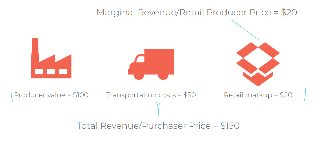
Below is an example to show how a purchase is allocated with Margins. Assume that a consumer spends $150 at a retail store. A portion of that price, $20 in this case, is retained by the retailer. Another portion, $30 goes to transportation costs, and $100 goes to the producing Industry that actually made the item.
The only Industries that can be margined in IMPLAN are retail and wholesale. Nearly all Commodities, on the other hand, can be margined. This file shows the 2018 Margins for Industries and Commodities.
INDUSTRY EVENTS
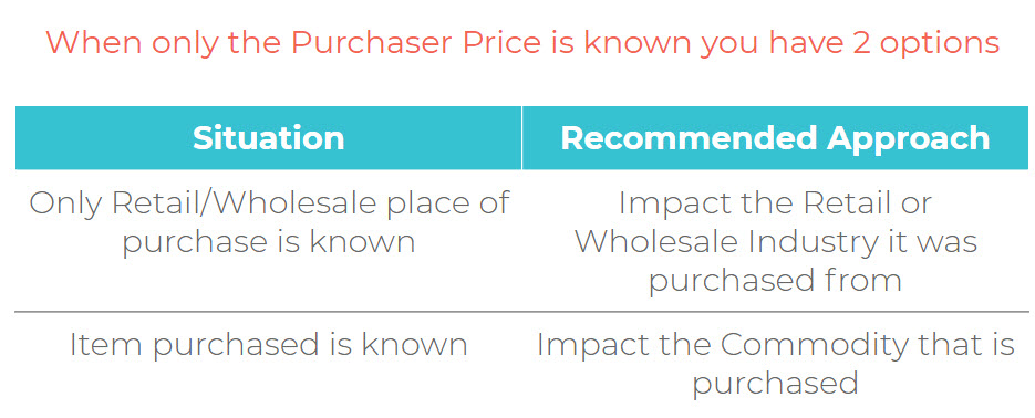
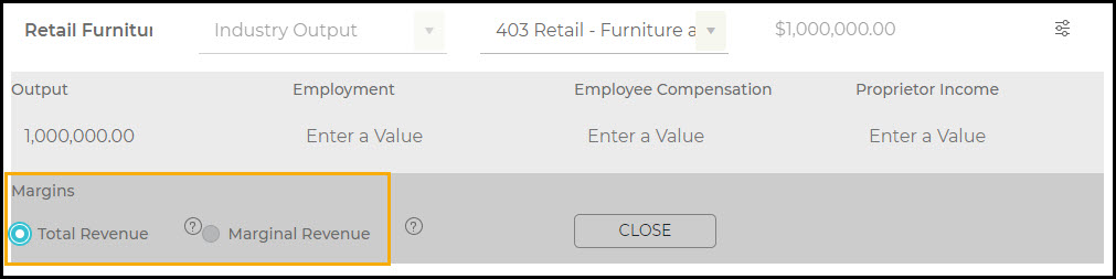
This feature is only available for retail and wholesale Industry Events. To apply margins for an Industry Event, open the menu. Here you will have the option to choose between Total Revenue (Purchaser Price) and Marginal Revenue (Producer Price). Most times, we only know the Purchaser Price, so leaving Total Revenue selected is the right choice. The Results in this case will only show the retail margin and its impact. Your Direct Effect to the retail Industry will be smaller than the Total Revenue you entered on the Impacts screen. All of other pieces of the value chain are lost (production, transportation, and wholesale).
If Marginal Revenue was chosen, the full $1M would be the Direct Output in your Results. This implies that you are modeling what the retailer is keeping (instead of just a portion of the item cost).
COMMODITY EVENTS
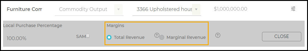
To apply margins in a Commodity Event, open up the menu icon and select between Total Revenue (Purchaser Price) and Marginal Revenue (Producer Price). Again, we usually know the Total Revenue, so the default selection is fine. The Results in this case will show us the impacts on the entire value chain for this Commodity; production, transportation, wholesale, and retail, with Direct Effects in each (when applicable).
If Marginal Revenue was chosen, you would again expect to see the full $1M applied to the Commodity 3366. The only deduction you might encounter is if some of the product was taken from inventory or produced by the government.
DEFLATORS:
Deflators are used to adjust for relative price changes over time. Output deflators are Industry specific and are used to adjust Industry Output. GDP deflators are not Industry specific and are used to adjust Final Demand and Value Added. Output and GDP deflators from the BEA are used for all past years, while BLS output deflators are used for future years.
The Bureau of Economic Analysis (BEA) provides historical Output deflators which we use for past to current years. The BEA Output deflators are provided with the BEA Gross Output data.
The BEA also has historical GDP deflators which we use for past to current years. The BEA GDP deflators come from NIPA Table 1.1.9 – Implicit Price Deflators for Gross Domestic Product. The BLS produces time-series of Output estimates for its Employment Growth Model. The Outputs are projected in real and constant dollars. This gives implicit price index projections which are the basis for projections of the IMPLAN deflators.
Both the BEA and BLS deflator data have fewer Industries than the IMPLAN Industry scheme; therefore, all IMPLAN Industries within a single BEA or BLS Industry will have the same deflator. This file shows the 2018 Deflators for Industries and Commodities.
DETAILED INFORMATION:
The purchasing power of a dollar changes over time (typically decreasing) due to inflation, a cyclical phenomenon by which prices of goods and services increase[1], which spurs workers to demand higher wages, which in turn increases demand for goods and services, thereby spurring additional price increases, and so on. Due to inflation, a dollar in 2017 cannot purchase as much as did a dollar in 2001, for example; as such, a 2017 dollar is not the same thing as a 2001 dollar. IMPLAN’s deflators are indexes of inflation, with the deflator for the model data year set at 1.00.
The deflators are not used to create the social accounts or multipliers but are necessary for impact analysis whenever the Dollar Year of the event differs from the Data Year being used. The same model year multipliers are used regardless of the Dollar Year of the event; it is the value applied to those multipliers that changes when the Dollar Year of the event differs from the Data Year.
All the relationships in the multipliers are based on model year prices, so the Direct Effects applied to those multipliers need to also be in the correct Dollar Year – this is accomplished via the deflators. The value applied to the multipliers is the user-entered value divided by the deflator. The deflators also allow impact results to be viewed in years other than the model year, regardless of whether or not the Dollar Year of the event differs from the Data Year.
While the Event values and/or result values can be inflated or deflated, depending on whether the index value being applied is less than 1.00 or greater than 1.00 (i.e., depending on the Industry or Commodity and whether one is adjusting to a future or past value), we use a single term – deflators – to refer to all of these index values.
The Output deflators are specific to the Industry or Commodity and are applied to the Output value, while GDP deflators are the same for every Industry and Commodity and are applied to all of the value-added components.
Margins are derived from the Bureau of Economic Analysis Input-Output tables. Margins are particularly important for Personal Consumption Expenditures (PCE) values as nearly all household purchases of goods are through a retail Industry. The Margins used to form the PCE data elements are compiled from the BEA Detailed Benchmark tables. This data provides the Margins associated with each of the different Personal Consumption categories. These PCE categories are modified to fit IMPLAN Industry definitions.
DOLLAR YEAR & DATA YEAR:
By default, impacts will be reported in current year dollars; however, because IMPLAN data are typically lagged a year (i.e., 2018 data were released in 2019), it is handy to be able to report the results in current year dollars. This can be achieved by changing the Dollar Year on the Results screen. This is just an option, and is not the same thing as changing the Dollar Year on the Impacts screen. The Dollar Year must match the year that the dollars represent – this ensures that the correct value is applied to the multipliers.
Suppose you are going to model the impact of the 500,000 visitors that came to your tourist attraction in 2020. Also suppose that you didn’t conduct your own visitor expenditures survey and are thus borrowing a survey that was conducted on a similar tourist attraction in a similar region but way back in 2010. That survey gives you the per-tourist expenditures on things like lodging, food, transportation, and entertainment. For example, each tourist spent $200 on lodging during their 3-night trip to that attraction. If you were to set Dollar Year to 2020 and put in $200 you would be understating your impact because 3 nights at a similar hotel would cost more than $200 in 2020 due to inflation! So you’d want to set the Dollar Year to 2010, since that is the year that those $200 represent. IMPLAN will inflate accordingly and apply the value to the multipliers.
Margins represent the value of the wholesale and retail trade services provided in delivering commodities from producers’ establishments to purchasers. This file contains the four components of the Value Chain: retail, wholesale, and transportation margins for each Industry along with the Producer value.
Deflators are used by the software whenever the Event Year is set to a year that differs from the model Data Year. This file has the deflators/inflators for 1997-2060.
IMPLAN data is updated annually, but the ‘current’ year lags behind the current calendar year. However, the data is a snapshot of the economy for the base year of the data set, the year for which the data was reported. Thus a 2004 Model of Orleans Parish will show the economy of 2004 (pre-Katrina) and a 2006 Model of Orleans Parish will show the economy of 2006 (post Katrina).
Here are a few interesting facts about the annual IMPLAN updates :
New data sets are released around the end of each calendar year and are a little more than a year behind that calendar year (e.g. 2013 was available at the end of 2014 and 2014 data was available around the end of 2015).
Data sources used to calculate the IMPLAN Data do not become available until early June of the following year (so data on the calendar year of 2013 was not begun to be released until June of 2014). Once the data sources become available, our Ph.D. economists and data developers begin compiling and converting this information into our unique IMPLAN data products.
This process includes:
Estimating non-disclosures
Converting Data to the current BEA Sectoring scheme
Projecting some data elements whose release date lags
Combining regional data sources and balancing reports from multiple sources so that sub-regions are forced to sum to the totals of their larger geographies (e.g. ZIP Codes sum to counties, counties to states, and states to the U.S.)
Creating trade estimates
Our data is derived from numerous sources, primarily federal agencies who conduct annual data collection and estimates, such as:
U.S. Bureau of Labor Statistics (BLS) including CEW and Consumer Expenditure Survey
U.S. Bureau of Economic Analysis (BEA) including REA data, Benchmark I/O accounts, and Output estimates
U.S. Census Bureau County Business Programs (CBP) and Dicennial Census and Population Surveys
U.S. Department of Agriculture Census
To investigate further into IMPLAN data sources please follow this link.
https://implan.com/wp-content/uploads/Market-site-Logo-resized-2-1.jpg00Joe Demskihttps://implan.com/wp-content/uploads/Market-site-Logo-resized-2-1.jpgJoe Demski2019-10-25 15:18:532019-10-25 15:19:05IMPLAN Annual Data Updates
Databases are available for the U.S., all 51 states (includes Washington, D.C.), 5 US Island area territories, and all 3,000+ counties in the United States. 30,000+ zip code level files are available. We also have a number of international data sets. You can view information on data selection on our website.
All IMPLAN datasets come in .ODF format and include a set of national I-O matrices and tables that allow the software to create a complete set of regional social accounts. Each U.S. data file – whether you are working at the zip code, territory, state, or national level – includes economic and demographic variables at a 536* industry/commodity sector level (defined by NAICS). Data variables include employment, income, taxes, and transactions by governments and households.
IMPLAN databases are constructed exclusively by IMPLAN Group LLC. IMPLAN has U.S. data available from 1996 forward. For trade flow estimate, we provide a National Trade Model for 2007 data sets and newer for US states and counties. Previous data years, US territories, and zip code files require use of the Econometric RPC trade flows method. National models (US and foreign countries) have foreign imports and exports pre-defined as part of the data base.
Additionally, all IMPLAN data sets include the software and data to build complete Regional SAM Multipliers. The software also provides a framework to easily perform impact analysis and creates reports for analyses and virtually all data elements.
For 2007 and later data, Trade Flow data are included with your annual database (in the Version 3.0 system only). The Trade Flow data available for county level and higher data sets provides all the tools necessary to build Multi-Regional I-O (MRIO) models, whether you are looking at flows between counties, between states, or between aggregated model regions. Currently, the MRIO functionality is only available in IMPLAN Pro.
*Number of sectors depends on the data year. For US files 2013 (and later), data sets are 536 sector; 2007-2012 are 440 sector; 2001-2006 are 509 sector and 1996-2000 are 528 sector.
Certain IMPLAN Sectors require additional explanation, either because they are not NAICS based or they have special properties. Below are the special Sector descriptions (sector numbers are based on the 536 sector scheme for 2013 and later IMPLAN data sets)1.
SECTORS 52-64: CONSTRUCTION
IMPLAN construction Sectors are classified by structure type (Census definitions) rather than NAICs codes. For this reason, Sector searches for construction will not pull up corresponding IMPLAN Sectors. Thus, when working with Construction Sectors, the Construction Codes for 536 Sectors spreadsheet on the IMPLAN website can be helpful.
SECTOR 441: OWNER-OCCUPIED DWELLINGS
IMPLAN Sectors 1-517 are private Sectors that directly correspond to the NAICS codes, with the exception of construction (see above) and Sector 441- Imputed rental activity for owner-occupied dwellings. This Sector estimates what owner/occupants would pay in rent if they rented rather than owned their homes. This Sector creates an industry out of owning a home, and its production function represents repair and maintenance of that home. The Sector’s sole product (Output) is ownership and is purchased entirely by personal consumption expenditures (i.e., the household Sector).
There is no Employment or Employee Compensation for this industry. Taxes on production for this Sector are largely made up of property taxes paid by the homeowner, while Other Property Income is the difference between the rental value of the home and the costs of home ownership. Interest payments and mortgage payments are a transfer in the SAM and are not part of the production function for this Sector.
Sector 441 is included in the database to insure consistency in the flow of funds. It captures the expenses of home ownership such as repair and maintenance construction, various closing costs, and other expenditures related to the upkeep of the space in the same way expenses are captured for rental properties.
SECTOR 517: PRIVATE HOUSEHOLDS
While not a true special Sector, there are often many questions regarding what Sector 517 produces. This sector covers live-in household staff: maids, butlers, chauffeurs, etc. If there is ever any question about what is covered by any of the “non-special” sectors, the user can use the sector definitions found in the Sector Search feature located in the Help menu of the desktop software (IMPLAN Pro) or within the event window in IMPLAN Online. Sort by clicking the the “NAICS Code” field header and scroll down to the IMPLAN sector of interest.
SECTORS 518-526: GOVERNMENT ENTERPRISES
IMPLAN Sectors 518-526 represent government agencies that cover a substantial portion of their operating costs by selling goods and services to the public. They operate much like private sector firms, hiring labor and purchasing other inputs to produce goods that are sold through markets. Other Federal\State\Local government enterprises (i.e., those other than postal, electric utility, and transportation services) include things such as government owned and operated liquor stores, airports, sewer and sanitation services, gas, and water supply2. This differs from Administrative Government sectors (components of consumption – i.e., final demand), because administrative do not respond to local market demands.
SECTORS 527-530: COMMODITY ONLY SECTORS
IMPLAN Sectors 527-530 are commodities not produced intentionally by any US industry:
Scrap consists of commodities that are cast off as part of a production process and then resold. Examples include sales of used aluminum cans to recyclers and sales of scrapped vehicles to metal recyclers.
Used and secondhand goods are goods that are traded but were not produced during the current year. While used goods are not part of the current-period gross output of the economy, they are part of the supply available for consumption. They come from capital, government institutions, and households.
Rest of world adjustment “The rest-of-the-world adjustment to final uses consists of values for exports and imports that have offsetting adjustments to personal consumption expenditures (PCE) and government… This adjustment is required in order to conform the commodity treatment of the I-O use table to the expenditure concepts used for final uses in the NIPAs. This is accomplished by making offsetting adjustments between PCE and gross exports and between Federal Government nondefense purchases and exports and imports…For example, foreigners traveling in the United States consume goods and services, such as accommodations, that are included in the source data for PCE. In order to put the PCE estimate on a NIPA basis, an adjustment is made to account for these purchases.”3
Non-comparable foreign imports are goods that are not available anywhere in the nation. They consist of three types of services: (1) services that are produced and consumed abroad, such as airport expenditures by U.S. airlines in foreign countries; (2) service imports that are unique, such as payments for the rights to patents, copyrights, or industrial processes; and (3) service imports that cannot be identified by type, such as payments by U.S. companies to their foreign affiliates for an undefined basket of services.
SECTORS 531-536: ADMINISTRATIVE PAYROLL SECTORS
Administrative government activities (e.g., legislatures, police protection) are not subject to local market forces (i.e., not driven by local demand); as such, they are held exogenous to the multiplier model.
IMPLAN Sectors 531-536 represent the payroll/value added of these administrative government Sectors. This is necessary because, while the commodity purchases of these government institutions are already represented in the SAM, there is no payroll commodity; thus, these four Sectors are included as a bookkeeping element to account for these institutions’ payrolls. By definition, these Sectors have no intermediate purchases and thus will not generate indirect effects. For these sectors, Employee Compensation or Employment should be used as Event values; entering the operational value of the government as an Industry Sales value will greatly overestimate the impact. When modeling government programs or budgets, you will need to import the appropriate spending pattern(s) associated to the budget activity. For public education budgets, the private educations Sectors (472-474) can often be used as adequate proxies as an alternative to importing the spending pattern.
NON-SECTORS: GOVERNMENT INSTITUTIONS
Government Institutions in IMPLAN do not have Sector designations. Instead these spending patterns are found in the Setup Activities screen by selecting Activity Options>Import>Institutions Spending Pattern in IMPLAN Pro or by selecting Import>Institutions Spending Pattern from the Activities page in IMPLAN Online. The following governmental spending patterns are available.
Federal Non-Defense: Spending pattern for all other government institutional activities.
Federal Defense: Spending pattern for the Department of Defense.
Federal Investment: Includes construction, equipment purchases, and other capital outlays. The U.S. total federal investment data comes from NIPA. This data is broken out with two additional data sets: a) the Annual Census of Construction and b) latest BEA BM-IO.
State/Local Government Non-Education: Parks & recreation, Health, Hospitals, Police, Judicial and legal, Financial administrative, Highways, Public welfare, Fire protection, Natural resources, Corrections, Libraries, Social insurance.
State/Local Education: Elementary and Secondary instruction, Elementary and Secondary non-instruction, Higher Education instruction, Higher Education non-instruction.
State/Local Investment: Come from the Census of State & Local Government Finances. These figures are adjusted so that the sum of states = the U.S. NIPA total State/Local Government Investment. The breakout of this figure comes from a) Annual Census of Construction and b) latest BEA BM I-O.
1 The IMPLAN Sectors discussed in this document correspond to IMPLAN’s 536 Sectoring scheme, in place since 2013. A bridge from the older 440 Sectoring scheme to the 536 Sectoring scheme can be found in the downloads section of this website.
2 Post exchanges are a type of store operated at U.S. Army bases by the Army and Air Force Exchange Service. Post exchanges provide merchandise and services to military families and generate income for military programs that provide social services, recreation, sports, and entertainment.
3 Horowitz, Karen and Planting, Mark. Concepts and Methods of the U.S. Input-Output Accounts, United States Bureau of Economic Analysis, April 2009, pp. 7-9 to 7-11.
IMPLAN employment includes both wage and salary employees and self-employed persons in a region. Full-time, part-time and seasonal workers are measured to create an estimate of annual average jobs.
BLS Covered Employment and Wages (CEW) data, BEA Regional Economic Accounts (REA) data, and County Business Patterns (CBP) data are used in conjunction to create IMPLAN data because no one dataset provides enough information to create a complete IMPLAN database.1 In general, CEW data provide the county level industry structure for IMPLAN, while CBP data are used to make non-disclosure adjustments to CEW data. REA data are used as controls for data not covered by CEW and proprietors.
CENSUS COUNTY BUSINESS PATTERNS (CBP)
County Business Patterns (CBP) is a program run by the U.S. Department of Census. Employment numbers are a count of employees during the week of March 12. This is a point-in-time estimate and not an annual average.
Data at the 6-digit NAICS level of detail include: total number of establishments, total first quarter employment, first quarter current year and total annual payroll, and a breakdown of the number of firms for 12 different employment size classes. As might be expected with 6-digit level specification, there are significant disclosure problems. However, even when the sector data are non-disclosed, CBP provides the number of firms by employee size class. The CBP also excludes most government employees and farm sectors.
The CBP data give a picture of the industrial structure of a region and are used to adjust the CEW data for non-disclosure. There is a time lag, generally one year, between the current year and the most recent CBP data, but an industrial structure generally changes slowly over time. There are virtually no disclosure problems with the national-level CBP data.
BLS COVERED EMPLOYMENT AND WAGES (CEW)
The CEW dataset is one of the most important datasets used in IMPLAN database development. These data provide the industry structure for the states and counties and the “ground truth” for IMPLAN data. There can be many differences between CBP and CEW, but in the end, if wage and salary employment doesn’t exist in CEW, it won’t exist in IMPLAN data sets. The data are provided by the U.S. Department of Labor as part of the Unemployment Insurance Covered Employment and Wages Program.
The CEW dataset provides annual average wage and salary establishment counts, employment counts, and payrolls by county at the 6-digit NAICS code level. These data are collected from a federal/state partnership program. State employment services departments, as part of the Unemployment Insurance Program, collect the data and pass it to the U.S. Department of Labor. As a result, only establishments that pay Unemployment Insurance are captured, hence the name “Covered Employment”. Since these data only capture covered employees, the data set cannot capture self-employed persons, railway employment, religious organizations, military, elected officials, or any other establishments that have their own social insurance program and/or do not pay into the Unemployment Insurance program. Since most farm employment is self employment, CEW data misses much of the farm data. Farm data is supplemented with REA data.
BEA REGIONAL ECONOMIC ACCOUNTS (REA)
The final set of employment and income information is the Bureau of Economic Analysis’s (BEA) Regional Economic Accounts (REA) data. This dataset is the most inclusive available and provides information on sectors such as agriculture, construction, and railroads not directly available through CBP or CEW.
The REA data series also provides information on self-employment and proprietor income. The major drawback to these data is that they are only available at the 3-digit NAICS level for state and county income, and the 3-digit and 2-digit level for state and county employment. These data provide a means to estimate proprietor employment and income, allowing for completion of the IMPLAN labor income data. The information used in developing IMPLAN data in this section is the following:
3-digit State level wage and salary income – SA7 tables
3-digit State level wage and salary employment – SA27 tables
3-digit State level employee compensation (wage and salary plus other labor income and benefits) – SA06 tables
3-digit State level total income (wage and salary and self-employment) – SA05 tables
3-digit State level total employment (wage and salary and self-employment) – SA25 tables
3-digit County level total income (wage and salary and self-employment) – CA05 tables
3-digit County level employee compensation (wage and salary plus other labor income and benefits) – CA06 tables
2-digit County level total employment (wage and salary and self-employment) – CA25 tables
6-digit disclosed CEW state and county employment and income data aggregated to the 3-digit NAICS, BEA sectoring scheme (used to project the REA data to the current data year).
BEA employment and income data are also subject to non-disclosure rules; therefore, estimates are made for non-disclosed values.
SEPARATING COUNTIES FROM INDEPENDENT CITIES
Unlike the CEW and CBP data, which give information on all counties and independent cities in the U.S., the BEA has combined independent cities with their neighboring counties in their REA data series. In Virginia, there are currently 24 such combinations. In 1994 and earlier datasets, WI also had one of these combined regions. These regions require special processes to split into separate Federal Information Processing Standards (FIPS) counties.
Names of REA Counties and their Combined Cities and City ID
The 3-digit CEW employment and income data are used to proportion the REA data into its component counties with alternative proxies being used where CEW data are unavailable or incomplete.
1 Other data sources are used to augment the above-listed sources for some specific sectors that are not fully covered by the above-listed sources or where more current data or data with more geographic or sectoral specificity are available.
https://implan.com/wp-content/uploads/Market-site-Logo-resized-2-1.jpg00Joe Demskihttps://implan.com/wp-content/uploads/Market-site-Logo-resized-2-1.jpgJoe Demski2019-10-25 15:16:282019-10-25 15:16:41Data Sets Used to Create IMPLAN Employment Data
Federal Government expenditure, sales, and investment data come from the latest BEA benchmark I-O tables, adjusted to NIPA control totals for the current year. National-level values are distributed to states and counties based on employment and employee compensation in Federal Defense and Non-Defense at the state and county level.
The one exception is Federal sales of stumpage, which is defined to be the sales volume of timber harvested (which includes sawlogs and all convertible volume) from National Forest land, and thus represents sales activity of the U.S. Forest Service (USFS). The USFS provides unpublished timber sales data at the state and county levels to IMPLAN. The data is obtained from a database maintained by the Washington Office Timber Sale Accounting (TSA branch). The data consist of:
Normal distribution or revenues received by the USFS as a result of the timber sales.
Purchaser Road Credits (PRC) directly related to the stumpage volume.
Associated charges to purchasers not directly related to stumpage, including items such as road maintenance, slash disposal, and coop scaling.
STATE AND LOCAL GOVERNMENT EDUCATION AND NON-EDUCATION
We combine several data sources to get State and Local Government purchases and sales data. We start with values from the latest Census of Government (inflated to the proper year). We then replace any Census values with any available equivalent values from the Census Bureau’s annual State and Local Government Finances Survey.
These data are totals – i.e., they do not have commodity specificity. At the state level, the resulting data represents the purchases and sales of State Government and Local Government combined, whereas at the county level, the data represents Local Government only. The state-level State and Local Government combined data are given commodity specificity upon controlling to U.S. commodity-specific values, which come from the latest BEA Benchmark controlled to current NIPA control totals. These state-level commodity-specific State and Local Government values are then distributed to the counties based on employment.
Validating the database is an important final step in the data development process.
VALIDATION PROCESS
Once the national model is complete and balanced, it is checked thoroughly for errors. Models are built and multipliers generated. All values are distributed to the states and counties based on the procedures outlined here. Once the data have been distributed to the states and counties, an extensive validation process takes place. State and county models are built and evaluated. The data are also passed through a program that calculates ratios on every value in the database. Any outliers are examined and either documented or fixed if a program or data bug is the cause. Once this process is complete, the databases are released to the public. Users should always examine their study area and make changes if required.
FORCE ACCOUNT ADJUSTMENT
To conform to I-O accounting definitions, IMPLAN industry data are subjected to an adjustment. This adjustment is called the force account adjustment and is an attempt to keep production activities consistent across sectors. For example, some non-construction industries, such as mining, have a large construction component. The force account construction adjustment moves the construction activity from the mining sector to the appropriate construction sector. The net result is that mining values may be slightly smaller than published estimates and the construction values may be slightly higher. Construction sectors can have production functions very different than the Industry using the constructed elements. Another highly affected sector is Hotels and Lodging. Restaurant, retail, and gaming activities that take place in hotels are moved to their respective sectors, thereby reducing the Hotels and Lodging sector to ~70% of its original size.
By keeping the activities separate, expenditures made during production will be more accurately allocated.
Regional Social Accounting Matrices, or SAM, represent an IMPLAN extension for regional Input-Output modeling. The SAM provides information on non-market financial flows. IMPLAN inter-industry models provide information on market transactions between firms and consumers, and they capture payments of taxes by individuals and businesses, transfers of government funds to people and businesses, and transfer of funds from people to people.
IMPLAN Group, LLC has developed methodologies for creating local (county) area SAM data that is consistent with Bureau of Economic Analysis’ National Income and Produce Accounts (NIPA).
SAM FRAMEWORK
Like Input-Output (I-O) tables, a full SAM is a double-entry bookkeeping system capable of tracing monetary flows between industries through debits and credits similar to T-Accounts in basic financial accounting. SAMs extend traditional I-O accounts by also providing information on non-market financial flows – i.e., industry-institution transfers and inter-institution transfers.
The matrix format allows the double-entry bookkeeping to be displayed in a single entry format. The column entries represent expenditures (payments) made by the economic agents. The row entries represent receipts or income to agents. By accounting definition, all receipts must equal all expenditures. That is, the SAM must balance. The shaded areas in Figure 24-1 are the inter-institutional (non-industry) transfers cells.
Column and row entries represent different economic actors. Across the row, “Industry” represents Industries producing goods and services. “Commodity” is the goods and services consumed by Industries and Institutions. “Factors” are factors of production, such as Employee Compensation, Proprietors Income, and Other Property Income. “Institutions” include Household and government accounts. “Capital” is investment and borrowing. “Enterprises” represent the distribution of corporate profits. “Trade” (exports and imports) show monetary flows into and out of a region.
Individual elements within the SAM tables include the use and make matrices and Value Added. The use table shows the use of Commodities by Industry or the goods and services required to produce an Industry’s output. The make table shows the make of Commodities by Industry, or who produces Commodities. These are typical components of Input-Output models. Also found in typical I/O models are final demand or Institutional consumption, exports, and imports.
The SAM adds non-industrial financial flows in addition to the typical I/O elements. Looking first at receipts or income, Industries make payments to Commodities for goods and services, payments to workers, profits (factors), payments to Institutions (households, governments, capital) or distributions, taxes, and borrowing. Lastly, Industries make payments to imports for use in production. The total is Total Industry Outlay.
Commodities make payments in the sense that there is a sum paid to produce Commodities. There are also non-Industrial sales of Commodities from Institutions.
Institutional income is also distributed to other Institutions. This is the real contribution of a SAM. These inter-institutional transfers show the flow of non-industrial funds. Inter-institutional transfers include transfers from businesses to households (interest and dividend payments), transfers from people to government (payment of taxes), and transfers from governments to people (social security, unemployment compensation, and other refunds and benefits). Inter-institutional transfers also include the capital accounts. For businesses, this is investment and borrowing. For households, this is net savings. Government capital accounts show surplus and deficits.
https://implan.com/wp-content/uploads/Market-site-Logo-resized-2-1.jpg00Joe Demskihttps://implan.com/wp-content/uploads/Market-site-Logo-resized-2-1.jpgJoe Demski2019-10-25 15:13:222019-10-25 15:13:35Introducing the SAM