Wage & Salary income includes base salary and/or wages, employee paid social insurance tax, bonuses, stock options, severance pay, profit distributions, and reimbursements for meals and lodging. It is a portion of Employee Compensation.
https://implan.com/wp-content/uploads/Market-site-Logo-resized-2-1.jpg00Joe Demskihttps://implan.com/wp-content/uploads/Market-site-Logo-resized-2-1.jpgJoe Demski2020-08-12 11:27:052020-08-12 11:27:05Wage & Salary Income
IMPLAN now includes data for occupation employment, wage, and core competency (knowledge, skills, abilities, education, work experience, and on-the-job training levels for each occupation). This new data offering allows for expanding employment impact results to include occupation detail (with associated wage, education, and skill detail) in addition to Industry detail. These data are also applied to the IMPLAN study area data, providing important insights into a Region’s existing skill force, the skill requirements of various industries, and more.
This article describes the methods and sources the IMPLAN Data Team uses to estimate these occupation and core competency data.
DATA SOURCES
There are four main sources for the IMPLAN Occupation Data. The most recent data years for each are utilized.
Bureau of Labor Statistics (BLS) Occupational Employment Survey (OES)
Provides data on knowledge, skills, abilities, education, work experience, and on-the-job training by occupation.
A new database version is released whenever updates are made.
For all sources, IMPLAN uses the most recent data release as of the time the occupation data generation process begins.
Occupation Data Year
OES
BLS
PUMS Data
O*NET
2018
2018
2018
2018
24.2
OCCUPATION EMPLOYMENT & COMPENSATION
It is important to note that IMPLAN reports occupation data only for the Wage and Salary Employment component of Total Employment, and therefore only for the Employee Compensation component of Labor Income. Note that proprietors are excluded from occupation-related IMPLAN data. This maintains consistency with Occupational Employment Statistics (OES) coverage only of “employees.”
OES data on occupation employment and wages by industry generally are available on an annual basis. IMPLAN relies most heavily on this dataset for occupation employment and compensation. The raw OES data report employment and wages by BLS SOC code, which has a hierarchy similar to North American Industrial Classification System (NAICS) codes. The SOC hierarchy occurs in 4 levels: major, minor, broad, and detail. OES data sometimes omit a level in the SOC hierarchy, e.g., reporting positive values at the detail level and its broad parent level, but nothing at the corresponding parent minor level. OES data also contain suppressions due to non-disclosure rules, with the result that a broad level code with 10 employees might report only one child detail code with 7 employees, leaving no information about the occupations of the remaining 3 employees.
When estimating occupation employment by industry, IMPLAN estimates values where that value would be non-disclosed in the OES data and ensures consistency among levels. That is, if 2 detail codes contain 5 employees each, the corresponding broad code will have 10 employees. Sometimes this requires overwriting published values that are inconsistent with other published values while ensuring that the IMPLAN data maintain as much consistency with the raw data as possible. IMPLAN’s method of disclosing missing values entails using data from aggregations at a higher NAICS or SOC level, as well as controlling lower-level values to known higher-level aggregates. Wage values are treated similarly to employment values in the disclosure process.
IMPLAN matches the disclosed and consistent occupation by industry employment data to IMPLAN Industries. In some cases, OES does not provide any coverage of an industry, such as agriculture and private households. In this case, IMPLAN supplements the OES data with data from the BLS Employment Projections, which also provide data on occupation employment by industry, but not on occupation wages by industry. Wage data from OES are substituted in this case. IMPLAN uses other BLS data to estimate military occupation employment, and deviates from the SOC system for coding military occupations. Occasionally, OES provides detail only to a NAICS level that encompasses more than one IMPLAN Industry. In such cases, IMPLAN applies the distribution of occupation employment for that NAICS code to all constituent IMPLAN Industries. Additionally, there are cases in which IMPLAN refines initial occupation estimates for an IMPLAN Industry that uses occupation data for an aggregate NAICS by accounting for a sibling industry that uses occupation data for a more detailed level of the same aggregate NAICS.
IMPLAN uses the occupation hours data from PUMS to adjust its estimates of occupation wages. The OES data on wages by occupation assume that each occupation works 2,080 hours per year (40 hours * 52 weeks), except in some cases in which it provides only an hourly wage. If IMPLAN followed that assumption, it might attribute too much compensation to occupations that tend to work fewer than 2,080 hours per year. For example, consider a hypothetical restaurant industry that has only one business. That restaurant has one waiter position, which is hired all year long but only for 20 hours per week and is paid $10 per hour. The waiter position should not be assumed to earn $10 * 2,080 = $20,800 per year; rather, the waiter would earn $10 * 2,080 * (20 / 40) = $10,400 per year. If this business also employs a restaurant manager, who works 40 hours per week and earns $20 per hour, the manager earns a total of $41,600. Properly accounting for hours worked means that the manager earns 80% of the total compensation paid by the business and in the industry, with the waiter earning the remaining 20%. Failing to account for hours worked gives the manager 67% and the waiter 33%.
CORE COMPETENCIES
KNOWLEDGE, SKILLS, ABILITIES, EDUCATION, WORK EXPERIENCE AND ON-THE-JOB TRAINING
Developed by Philip Watson, Ph.D.
Each occupation in IMPLAN is deconstructed into their constituent Knowledge, Skill, and Ability (KSA) elements as well as education levels, work experience, and on-the-job training using Bureau of Labor Statistics (BLS) data and O*NET™ data. The KSAs along with education, experience, and training are referred to as the “core competencies.”
O*NET™ data report 33 unique knowledge elements, 35 unique skill elements, 52 unique ability elements, 12 unique educational attainment elements, 11 unique work experience levels, and 9 unique on-the-job training levels. Descriptions of these core competency elements can be found in the Core Competencies spreadsheet.
In order to generate workforce reports, IMPLAN occupation data must be bridged to the core competencies. However, neither O*NET™ databases nor the BLS provides a bridge between occupations and core competencies; rather, they report values on two scales for each occupation and KSA combination. The scales that are reported are a 0-5 measure of “importance” and a 0-7 measure of “level.” Combining these two scales into a bridge of occupation employment to measures of KSA endowments requires some assumptions and empirical calculations. The assumptions used, while not intended to be regarded as the only set of assumptions that could be used to generate the bridges, were empirically tested to ensure that the resulting bridges accurately predicted occupation wages and presented a reasonable measure of the KSAs associated with each occupation.
ASSUMPTIONS
The first assumption used in generating the bridges is that the two KSA scales would be combined using a multiplicative interaction between the scales. The use of a multiplicative relationship rather than an additive interaction deemphasizes very small values for either the level or the importance and creates a higher weight for KSA elements that have higher values for both the level and the importance. Alternative interactions were also explored, including additive, arithmetic means, and geometric means, but the multiplicative interaction was found to be the best across multiple empirical tests.
The second assumption is that core competency endowments are associated with the occupations to which people are employed (or potentially unemployed) in a region rather than directly to the people themselves. Therefore when a person moves from one job to another within a region, the core competencies in the region change even though the same people reside and work there as before. More technically, the core competencies generated here are a measure of the expected human capital endowments in the region given the current occupation mix of employment in the region. This assumption relates directly to the third assumption below.
The third assumption in generating the bridge is that every occupation uses the same absolute amount of KSAs and, therefore, the differences between the KSAs associated with different occupations are in their distribution, not their level. This assumption is useful due to the incompatible units across KSA elements. The result of this assumption is that every occupation can be thought of as using 100 units of knowledge elements, 100 units of skill elements, and 100 units of ability elements in varying distributions. When a worker moves from one job to another, the worker’s mix of KSAs change, but the overall amount of total KSAs which the worker possess does not change. Likewise, under this assumption education and training do not necessarily increase the absolute level of KSAs in a region; rather, they simply enable people to move from one occupation to a different occupation with a different (and presumably more valuable) set of associated KSAs.
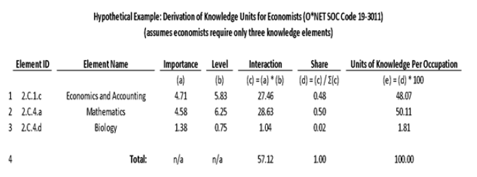
The chart below presents a numerical example of calculating units of knowledge elements from the O*NET data. The example is simplified, as O*NET includes many more knowledge elements for the economist occupation. According to this example, if an economy contains only one job, and that one job is held by an economist, the economy would have 100 units of knowledge, allocated among the three types listed below. The calculation is the same for other occupations and for other KSA types.
The other core competencies outside of the KSAs were more straightforward in their bridging to occupation data. Education, work experience, and on-the-job-training data from the O*NET™ database are reported as proportions of persons employed in a given occupation that each have a given level of education or training, respectively. O*NET™ data report 12 levels of educational attainment, 11 levels of work experience, and 9 on-the-job-training categories. Since they are already reported as proportions, the bridge to IMPLAN occupation data is direct and does not require any additional assumptions. The education, work experience, and training categories can also be found in the Core Competencies spreadsheet. However, similar to the KSAs, the education and training elements are occupation-based and not individual-based; therefore, they are not to be thought of as the direct endowments of the individuals in a region, but rather as the expected endowments relative to the occupation employment in the region.
While O*NET data covers the majority of OES occupations, there are occupations in the O*NET database that lack data. For example, the “all other” occupations (SOCs ending in 9: xx-xxx9) often lack O*NET data. In such cases, core competency data for the occupation is estimated using the core competency estimates of sibling level occupations weighted by each competency’s survey response size as provided by O*NET. This approach assumes that the “all other” occupation reflects the competency emphasis of the sibling occupations. Additionally, military occupations were estimated using similar means in order to bridge O*NET data to IMPLAN’s custom military occupation codes.
Given the data and assumptions described above, IMPLAN can estimate endowments of the respective core competencies which will sum to 100 times the same total as the occupation employment total in the region. For example, if there are 1,000 occupation jobs in a given region, then there will be 1,000*100 occupation equivalents of knowledge, 1,000*100 occupation equivalents of skills, and 1,000*100 occupation equivalents of abilities. These occupation equivalents will vary widely by region based on the industrial and occupation employment mix in the respective region.
The data Behind the “i” is helpful for better understanding the Results produced in your analysis.
CALCULATION STEPS:
To calculate the leakages due to spending on Intermediate Inputs outside of the Study Region click on the “i” icon next to the Selected Region and navigate to:
Social Accounts
> Balance Sheets
> Industry Balance Sheet
> Commodity Demand
In the Commodity Demand table, you’ll find the following columns (be sure to filter by your Industry of interest):
Gross Absorption = the proportion of Total Industry Output for this industry that goes toward purchases of each commodity. Gross Absorption is calculated as Gross Inputs/Total Industry Output. Total Gross Absorptions will be less than one, with the remainder of Total Industry Output going toward Value-Added.
Regional Absorption = the proportion of Total Industry Output for this industry that goes toward local purchases of each commodity. Regional Absorption can be calculated as Gross Absorption * RPC
Therefore, Total Gross Absorption – Total Regional Absorption = percentage of Total Industry Output that is spent on Intermediate Inputs outside of the Region. This percentage multiplied by Total Industry Output are the Intermediate Input dollars leaked out from the Direct Effect.
Take for example “Industry 56 – Construction of other new nonresidential structures” in Pennsylvania 2018. The Total Gross Absorption is 52.057% and the Total Regional Absorption is 31.671%. This means about 52% of Output is allocated to Intermediate Inputs overall, and about 32% of Output is allocated to Intermediate Inputs in the Region. Therefore, about 20% of Output is allocated to Intermediate Inputs outside of the Region.
% of Total Industry Output spent on non-local Intermediate Inputs = 52.057% – 31.671% = 20.386%
When analyzing $1M of new Output in this Industry in PA, IMPLAN would estimate $203,860 of the $1M of new production as being spent on non-local Intermediate Inputs. The remaining $796,140 includes local Intermediate Inputs ($316,710) and Value Added ($479,430).
https://implan.com/wp-content/uploads/Market-site-Logo-resized-2-1.jpg00Joe Demskihttps://implan.com/wp-content/uploads/Market-site-Logo-resized-2-1.jpgJoe Demski2020-08-12 11:08:092020-08-12 11:08:09Calculating Leakages of Direct Intermediate Inputs
We get this question a lot at IMPLAN. You run an analysis of $5M and your Results only show $4.8M in Direct Output. Where did the other $200,000 go?
There are seven reasons that these numbers won’t match. Let’s walk through them.
THE SEVEN REASONS WHY
MISSING INDUSTRY
If you are modeling a list of Industries, it is possible that one of them doesn’t exist in your Region. If it doesn’t exist in the IMPLAN data, there will be no effect from that Industry. If you know that the Industry does now operate in your Region, you can add it by Customizing your Region.
DIFFERENT DOLLAR YEARS
In order to see the exact number that you used on the Impacts screen in your Direct Effects, you will need to ensure that your Dollar Year matches on both screens. For example, if you analyzed your Events using 2018 Dollar Year, filter your Results for 2018 Dollar Year. If different years are used, you will not see exact matches between the Impacts screen and the Results screen. Check out the article on Dollar Year & Data Year for more details.
EVENT TYPE
The only Event Types that will give you a Direct Effect are Industry Events, Industry Contribution Events, Commodity Output Events, and Institutional Spending Pattern Events. Direct Effects are not a part of Labor Income Events, Household Income Events, or Industry Spending Pattern Events. More details are in the article Explaining Event Types.
MARGINS
A Margin is the value of the transportation, wholesale, and retail trade services provided in delivering Commodities from the factory floor to buyers. Margins are calculated as sales receipts less the cost of the goods sold. They consist of the trade Margin plus sales taxes and excise taxes that are collected by the trade establishment.
Most Input-Output models, including IMPLAN, record expenditures in producer prices (known as Marginal Revenue). This allocates expenditures to the Industries that produce the goods or services. Any Output or sales you want to apply to multipliers that are in purchaser prices (prices paid by final consumers) need to be converted from purchaser price (Total Revenue) to producer prices (Marginal Revenue) or allocated to the producing Industries. Margins enable the move from producer to purchaser prices or vice-versa.
IMPLAN values are based on the actual costs of producing the product or service being sold. Margins are necessary whenever an item is purchased from a retailer or wholesaler. Margins can be applied to retail and wholesale Industry Events and Commodity Events.
When margins are applied, you will not see the full Value from your Impacts screen in your Results. The portion that you do see in the Results is the margin coefficient for retail or wholesale Industry. Details can be found in these two articles: Retail and Wholesale: Industry Margins and Retail and Wholesale: Commodity Margins.
LOCAL PURCHASE PERCENTAGE
The Local Purchase Percentage (LPP) in Commodity Output Events and Spending Pattern Events is by default set to 100%, but this can be edited via the Advanced Menu. Remember, the LPP indicates to the software how much the Event impact affects the local Region and should therefore be applied to the Multipliers. If the LPP is set to anything less than 100%, you won’t see your inputs match the Results. Learn more in the article Local Purchase Percentage (LPP) & Regional Purchase Coefficients (RPC).
COMMODITY MARKET SHARE
The portion of Commodity supply coming from each source for a given Commodity is called a Market Share. If you are analyzing Commodities, some of the Market Share can come from Institutional Sales (like out of inventory or produced by the government). When LPP is less than 100%, the remaining portion (or 1-LPP) is then assumed to be affecting a different Region. The portion happening outside the Region of your analysis does not create any local effect.
Because Commodity Market Shares allocated to Institutions will be treated as leakages, these portions of Commodity Output will not be included in the Direct Effect of the Results. Check out where to find the Market Shares in the article on Social Accounts.
COMMODITY EVENTS AND DEFLATORS/INFLATORS
When a Commodity Event is run with the same Dollar Year and Data Year and the Results are viewed in that same Dollar Year, the Direct Effect will match the Direct Commodity input. However, when the Dollar Year on the Impacts screen or the Dollar Year on the Results screen do not match the Data Year, the Direct Effect will be slightly different than the Direct inputs. This is because the Commodity Event is adjusted using Commodity deflators/inflators and then those dollars are deflated/inflated on the Results using Industry deflators/inflators. The slight difference in the Results you see in the Direct Effect is due to the differences between Commodity and Industry deflators/inflators.
https://implan.com/wp-content/uploads/Market-site-Logo-resized-2-1.jpg00Joe Demskihttps://implan.com/wp-content/uploads/Market-site-Logo-resized-2-1.jpgJoe Demski2020-08-12 11:02:282020-08-12 11:02:28Why don’t my Direct Effects match my Direct inputs?
The table below clarifies the underlying level of detail of all line items in an IMPLAN tax impact report. In principle, the tax impact report captures all tax revenue in the study area across all levels of government that exist in that study area for the specific industries and institutions affected by an event or group of events. The underlying data that support the tax impact report, however, do not embody that much detail.
For example, IMPLAN does not have systematic reports of state government tax revenue by county; IMPLAN has same-year state government tax revenue by state and must allocate that to counties based on proxy information (we do have county-level data for some states, and use this to build a model for the allocation process). Also, IMPLAN obtains detailed TOPI data by geography (even for each city within a county), but does not have any industry detail about the specific TOPI line item. A third note: for the data by city, we often must aggregate that to the county level, so that a model of two cities in the same county will have the same implied effective tax rates. In other words, city-specific data will be used, but averaged across all cities within a county.
Please note that all line items are controlled to nationwide, current-year controls estimated by the Bureau of Economic Analysis (BEA) in the National Income and Product Accounts (NIPAs) with no industry resolution and two level-of-government distinctions, Federal and State & Local. For example, the NIPAs might give a value of $15 billion in State & Local income tax in 2017, which would be reflected in the 2017 IMPLAN data.
Industrial and geographic resolution are reported at their maxima and nest more aggregate levels. For example, if IMPLAN has raw data on property tax at the county level, that implies we also have state-level data.
Timeliness lags are reported vis-à-vis the dataset year. For example, a 1 year lag for 2017 IMPLAN data means that the underlying data have a reference year of 2016. Timeliness is especially relevant for knowing whether changes in tax laws or economic conditions are reflected in the IMPLAN dataset.
The table below does not report the combined State & Local level of government, since (other than nationally in the NIPAs as explained above) IMPLAN does not collect any data at this level; it’s simply an aggregate for legacy and convenience purposes.
Level of Government
Tax Impact Item
Maximum Industry Resolution of Underlying Data
Maximum Geographic Resolution of Underlying Data
Timeliness of Underlying Data
City/Special District
TOPI: Property Tax
TOPI aggregate at BEA sectoring (approximately 80 sectors).
TOPI detail has no industry resolution.
County level
1-2 years lag
City/Special District
TOPI: Motor Vehicle License
TOPI aggregate at BEA sectoring (approximately 80 sectors).
TOPI detail has no industry resolution.
County level
1-2 years lag
City/Special District
TOPI: Severance Tax
TOPI aggregate at BEA sectoring (approximately 80 sectors).
TOPI detail has no industry resolution.
County level
1-2 years lag
City/Special District
TOPI: Other Taxes
TOPI aggregate at BEA sectoring (approximately 80 sectors).
TOPI detail has no industry resolution.
County level
1-2 years lag
City/Special District
TOPI: Special Assessments
TOPI aggregate at BEA sectoring (approximately 80 sectors).
TOPI detail has no industry resolution.
County level
1-2 years lag
City/Special District
Personal Tax: Income Tax
n/a
County level
1-2 years lag
City/Special District
Corporate Profits Tax
None
County level
1-2 years lag
City/Special District
Personal Tax: Motor Vehicle License
n/a
County level
1-2 years lag
City/Special District
Personal Tax: Property Tax
n/a
County level
1-2 years lag
City/Special District
Personal Tax: Other Tax
n/a
County level
1-2 years lag
County
TOPI: Property Tax
TOPI aggregate at BEA sectoring (approximately 80 sectors).
TOPI detail has no industry resolution.
County level
1-2 years lag
County
TOPI: Motor Vehicle License
TOPI aggregate at BEA sectoring (approximately 80 sectors).
TOPI detail has no industry resolution.
County level
1-2 years lag
County
TOPI: Severance Tax
TOPI aggregate at BEA sectoring (approximately 80 sectors).
TOPI detail has no industry resolution.
County level
1-2 years lag
County
TOPI: Other Taxes
TOPI aggregate at BEA sectoring (approximately 80 sectors).
TOPI detail has no industry resolution.
County level
1-2 years lag
County
TOPI: Special Assessments
TOPI aggregate at BEA sectoring (approximately 80 sectors).
TOPI detail has no industry resolution.
County level
1-2 years lag
County
Personal Tax: Income Tax
n/a
County level
1-2 years lag
County
Corporate Profits Tax
None
County level
1-2 years lag
County
Personal Tax: Motor Vehicle License
n/a
County level
1-2 years lag
County
Personal Tax: Property Tax
n/a
County level
1-2 years lag
County
Personal Tax: Other Tax
n/a
County level
1-2 years lag
State
TOPI: Property Tax
TOPI aggregate at BEA sectoring (approximately 80 sectors).
TOPI detail has no industry resolution.
State level
0 years lag
State
TOPI: Motor Vehicle License
TOPI aggregate at BEA sectoring (approximately 80 sectors).
TOPI detail has no industry resolution.
State level
0 years lag
State
TOPI: Severance Tax
TOPI aggregate at BEA sectoring (approximately 80 sectors).
TOPI detail has no industry resolution.
State level
0 years lag
State
TOPI: Other Taxes
TOPI aggregate at BEA sectoring (approximately 80 sectors).
TOPI detail has no industry resolution.
State level
0 years lag
State
TOPI: Special Assessments
TOPI aggregate at BEA sectoring (approximately 80 sectors).
TOPI detail has no industry resolution.
State level
0 years lag
State
Personal Tax: Income Tax
n/a
State level
0 years lag
State
Corporate Profits Tax
None
State level
0 years lag
State
Personal Tax: Motor Vehicle License
n/a
State level
0 years lag
State
Personal Tax: Property Tax
n/a
State level
0 years lag
State
Personal Tax: Other Tax
n/a
State level
0 years lag
Federal
Social Insurance Tax- Employee Contribution
None
State level
0 years lag
Federal
Social Insurance Tax- Employer Contribution
None
State level
0 years lag
Federal
TOPI: Excise Taxes
TOPI aggregate at BEA sectoring (approximately 80 sectors).
TOPI detail has no industry resolution.
National level
0 years lag
Federal
TOPI: Custom Duty
TOPI aggregate at BEA sectoring (approximately 80 sectors).
TOPI detail has no industry resolution.
National level
0 years lag
Federal
Corporate Profits Tax
None
National level
0 years lag
Federal
Personal Tax: Income Tax
n/a
National level
0 years lag
Federal
Personal Tax: Estate and Gift Tax
n/a
n/a
n/a
METHODOLOGY:
Initially, the estimation of value added by sector and taxes by level of government proceed independently.
Taxes by level of government are obtained by combining data from the Annual Survey of State and Local Government Finances, which usually is lagged a year or two with respect to the IMPLAN data reference year, the most recent state government tax collections (also reported by the Census Bureau), and the most recent Census of Government Finance, which is like the Annual Survey, but covers every single unit of government. Those sources report tax by type, by unit of government (ergo by level of government), and by location. State government revenue is assigned only at the state level (i.e., the data do not tell us how much state income tax came from a given county). Federal government revenue is known only at the national level from the National Income and Product Accounts.
Data for county, city, and special district governments are assigned to the counties containing those units of government. Data for state and federal government revenue are allocated to counties based on proxies (e.g., personal income by county is used to allocate state government personal income tax revenue to counties). We have national level controls for taxes by level of government and type of tax from the National Income and Product Accounts. We first distribute taxes to states using a combination of the combined finances data and data on total taxes by state (covering both state and local governments) from the BEA’s Regional Economic Accounts. We then distribute those state values to counties based on the combined finances data, where possible, and by proxies where not possible.
The only industry-level detail we have for taxes is for TOPI, and it is for the entirety of TOPI, not the components of TOPI (e.g., sales tax, property tax, etc.). The components are only place- and level-of-government specific, not industry-specific.
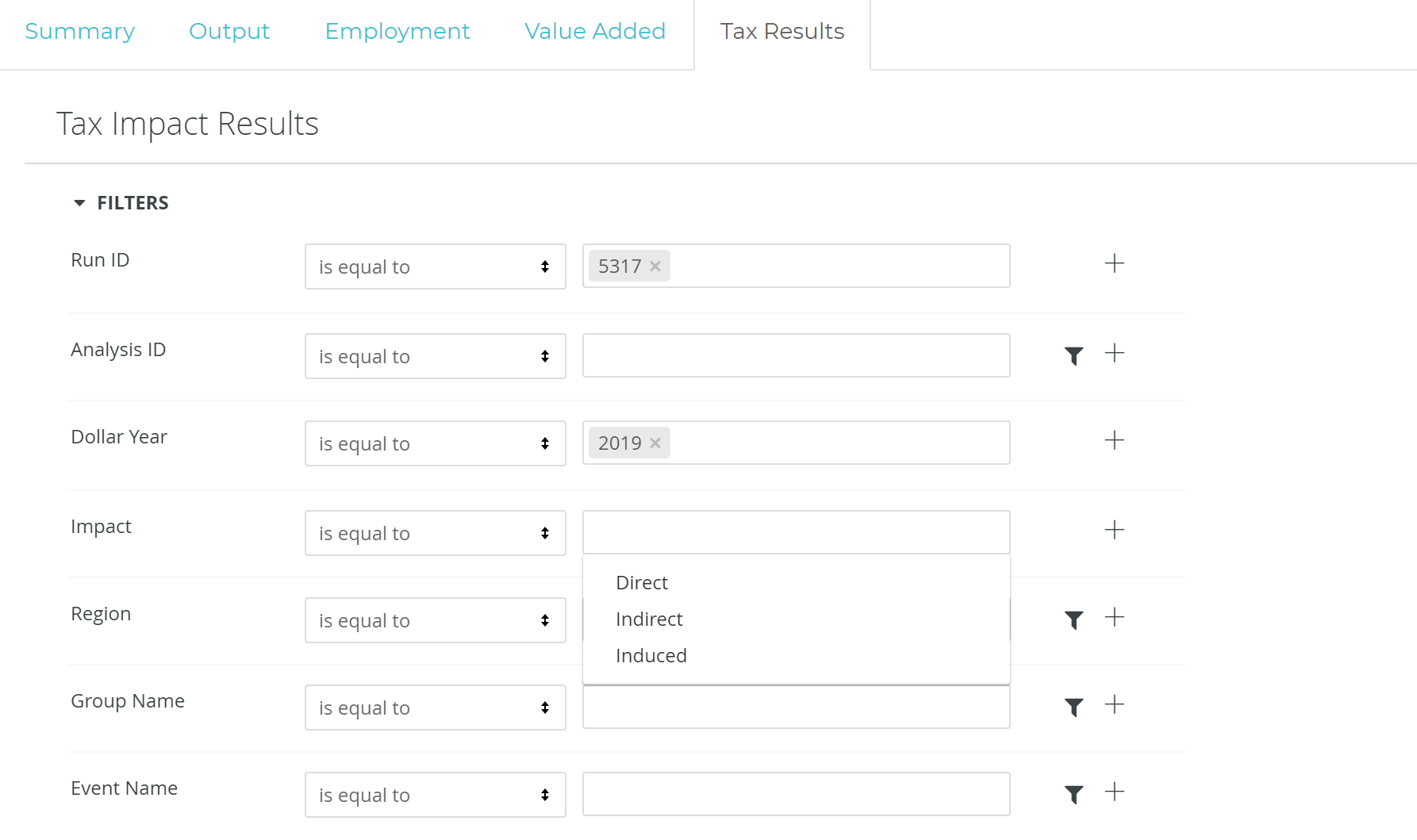
FILTERING:
To filter by Direct, Indirect, and Induced taxes in IMPLAN, simply open the Filter window and click into the “Impact” Filter. This will provide you the option of “Direct”, “Indirect”, “Induced”. Making a selection and clicking “Run” will apply the filter and only show the Tax Results as specified. if no selection is made, you are viewing total Tax Results.
Generation and Interpretation of IMPLAN’s Tax Impact Report
https://implan.com/wp-content/uploads/Market-site-Logo-resized-2-1.jpg00Joe Demskihttps://implan.com/wp-content/uploads/Market-site-Logo-resized-2-1.jpgJoe Demski2020-08-12 10:14:372020-08-12 10:14:37Generation and Interpretation of IMPLAN’s Tax Impact Report
Production functions detail the relationship between inputs and outputs. They represent the technically-efficient combination of inputs required for producing a certain level of output (Hess, 2002). This article outlines the three most common production functions, with an emphasis on our personal favorite, the Leontief Production Function.
PRODUCTION FUNCTIONS & ISOQUANTS:
In general, functions talk about relationships between variables.The basic formula for production functions is:
Isoquants are the lines shown in graphical representations of production functions that show the required financial capital (K) and labor (L) required to produce the quantity of output (Q). The ability to substitute factors of production is demonstrated in the shape of the isoquants (Hess, 2002).
There are three main types of production functions: linear, Cobb-Douglas and Leontief. The differences among them lie in the relationship between the variables: output, capital, and labor. The Leontief Production Function is used in IMPLAN to dictate the ratio of inputs needed by each Industry in order to produce a unit of Output (in terms of dollar value).
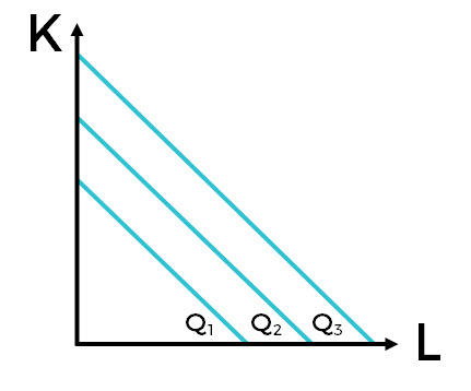
LINEAR PRODUCTION FUNCTIONS
The most basic is the Linear Production Function. Here, output is a simple function of inputs; unlike in the Leontief Production Function, capital can be substituted for labor perfectly. In the graph, we see three straight isoquants each showing the level of capital (K) and labor (L) required to produce the quantity of output (Q) (represented by the lines). In this equation, a and b are the output elasticities of K and L. Output elasticity refers to the ratio of change in Output to the proportionate change in input.
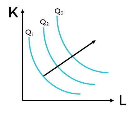
COBB-DOUGLAS PRODUCTION FUNCTION
The classical production function is commonly termed the Cobb-Douglas Production Function. Here, we see that output (Q) is still a function of capital (K) and labor (L), however, we also see the addition of a productivity assumption (A). Productivity is built into each Leontief Production Function within every IMPLAN dataset based on the level of productivity for the given Industry and Data Year. As with the linear production function, a and b represent the output elasticities of K and L.
The isoquants in the Cobb-Douglas Production Function are curved with the slope changing along them. This indicates that the capital and labor inputs are not perfect substitutes for each other. There can be input substitution, but it is not linear.
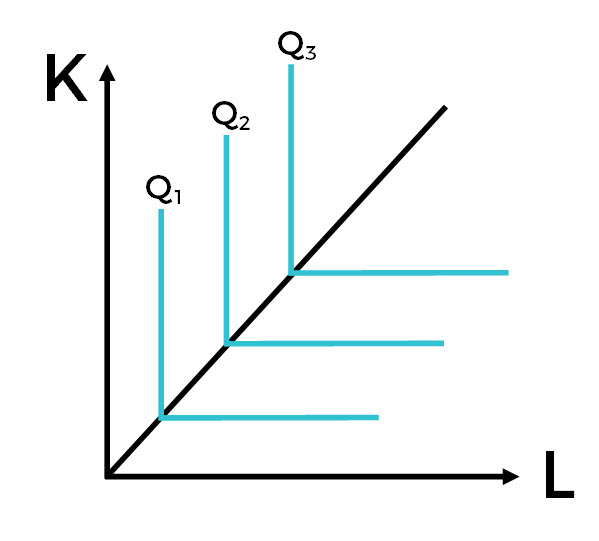
LEONTIEF PRODUCTION FUNCTION
The Leontief Production Function (LPF), named for the father of Input-Output economics Wassily Leontief, is what is utilized in IMPLAN. It is also known as the Fixed-Proportions Production Function. We still see output (Q) being a function of capital (K) and labor (L). The designation of min refers to the smallest numbers for K and L.
The isoquants in the LPF are right angles. Capital and labor are fixed proportions. They are perfect complements and cannot be substituted for one another. Increasing the inputs will lead to a proportional increase in output (Miller & Blair, 2009). Also, you can’t have too few or too many outputs; the relationship between capital and labor is locked.
THE LPF IN IMPLAN:
So that was a fun economics lesson, but how does this work in IMPLAN? Well, it all comes down to Output, the total annual production value of each Industry. The LPF of an Industry in IMPLAN determines how each Industry will allocate Output. Industries have employees, they pay Labor Income and Proprietor Income. They also pay taxes (Taxes on Production and Imports) and realize profits (Other Property Income). These combine to give us Value Added. In addition to the Value Added, Industries spend money on Intermediate Inputs.
Instead of just Output just consisting of capital and labor, we have an equation for Output that includes all of these pieces:
Note that while IMPLAN is based on the Leontief Production Function, you can make changes to Industry relationships using a technique called Analysis by Parts which allows for customization of the LPF.
Hess, P. (2002). Using Mathematics in Economic Analysis. Upper Saddle River, NJ: Prentice Hall.
Miller, R.E. & Blair, P.D. (2009). Input-output Analysis: Foundations and Extensions (second edition). New York: Cambridge University Press.
https://implan.com/wp-content/uploads/Market-site-Logo-resized-2-1.jpg00Joe Demskihttps://implan.com/wp-content/uploads/Market-site-Logo-resized-2-1.jpgJoe Demski2020-08-12 09:29:382020-08-12 09:29:38Understanding the Leontief Production Function (LPF)
When working with Zip Code level data, there are several factors to consider. This article, while not exhaustive, lists the main items to keep in mind when using Zip Code data for your geographical study Region.
AGGREGATION & LEAKAGES:
Zip code files, like other IMPLAN files, can be combined to create a Region or used independently. Please keep in mind that while an individual zip code file will create Multipliers and have impacts, these impacts will be minimal. This is because zip codes may have little or no population and/or little to no employment. Also, many individual zip codes are not large enough to allow for local sourcing of materials needed for the indirect effect or to provide adequate services to create significant induced effect leading to much of the potential impact being lost in leakages.
Zip code regions may represent very small economic Regions and consequently, be extremely open to leakages. These leakages, even to nearby regions (in some instances this could literally be across the street) are lost from the Region resulting in very small Indirect and Induced Effects. Please take into consideration where indirect purchases will be located and where employees may be spending their labor income when customizing zip code regions for analysis.
MRIO:
Multi-Regional Input-Output (MRIO) analysis allows for purchases to be made between Regions (the zip code(s) and the linked regions) by tracking trade between these regions, potentially capturing many of the lost impacts.
MISSING ZIP CODES:
Not all zip codes listed by the U.S. Postal Service may be represented in the zip code package you receive. The USPS can open/close post offices or reorganize routes on an on-going basis, thereby changing zip-code demographics. Because of this, the County Business Patterns and Census demographic zip code representation may not be current.
Depending on the year, roughly 4% of zip-codes have neither County Business Patterns (CBP) employment nor Census (demographic) data. If your region includes any of these zip codes, they will not be available in the package you purchase, as there is inadequate information to create Multipliers for these regions. Depending on the year, there will be roughly 8,000 zip-code files for which there is only CBP data with no demographic data. Most of these are P.O. boxes and “unique” point codes. They serve business but do not represent residential population. With no household representation, all employment would be considered in-commuting and have no local induced effect.
Conversely, there are also some zip-code files with only demographic data and no CBP data. While CBP data does not exist for these zip-codes, they may still contain employment in some sectors since CBP data do not cover all IMPLAN sectors. Population is used as a distributor for most of these non-covered sectors. Farm counts by zip-code from the 2017 Census of Agriculture are used to distribute agricultural industry data in these cases.
There will be cases where you may find an Industry exists in an actual zip code region but does not show up in the zip code data (or even the county data). This occurs because of unreported sectors in the CBP and inconsistencies in data between CBP and BLS covered wages and employment. When this issue occurs, you will need to customize your Region to add the Industry to the Study Area. CBP data are primarily obtained from administrative records supplied by the IRS, Social Security, and other sources. CBP is tabulated on an establishment basis, and each business location is tabulated only once according to the primary business activity. The industry classifications of establishments in the CBP are self-reported in the vast majority of cases. BLS CEW data are obtained from quarterly tax reports submitted to State Employment Security Agencies.
https://implan.com/wp-content/uploads/Market-site-Logo-resized-2-1.jpg00Joe Demskihttps://implan.com/wp-content/uploads/Market-site-Logo-resized-2-1.jpgJoe Demski2020-02-19 09:02:422020-02-19 09:02:53Understanding Zip Code Data
Are you interested in looking at IMPLAN data across years? Our Panel Data might be what you are looking for! It is produced using our latest and best methodologies, which have been improved over the past 20 years of data development. These enhanced features make more accurate statistical analysis possible. Panel Data consists of repeated measures on the same regions over time. In IMPLAN, we have data going back to 2001 that allows you to compare your Region and your Industry through time.
DATA SOURCES:
The Panel Data are the standard IMPLAN datasets. Each year a variety of data sources are compiled to create the IMPLAN datasets. Most of IMPLAN’s Industries are based on definitions put forth by the Bureau of Economic Analysis (BEA). For more information, visit the article IMPLAN Data Sources.
You’ll receive data files for Demographics, Industries, Commodities, and a file that contains deflators (as all data are presented in nominal dollars and not adjusted for inflation). This way you can quickly look at changes by Industry and Year for your geography to see how your economy is changing.
DEMOGRAPHIC DATA:
These data include, for each geography and year, population, land area, total personal income, the total number of households and the number of households by 9 income categories, and the Shannon-Weaver Index (S-W Index). Personal income includes not just labor income, but also personal dividend income, personal interest income, rental income of persons, and transfer payments. Labor income information can be found in the Industry Data file. The Shannon-Weaver Index is an index of economic diversity based on the distribution of employment among all sectors.
INDUSTRY DATA:
These data include, for each geography and year, each IMPLAN Industry’s Output, total Employment, Wage and Salary Employment, Proprietor Employment, Employee Compensation (EC), Proprietor Income, Other Property Income (OPI), and Taxes on Production and Income net of subsidies (TOPI).
COMMODITY DATA:
These data include, for each geography and year and Commodity, the Institutional level, the foreign exports of each IMPLAN Commodity from the region (via the Foreign Exports institution), foreign imports, each IMPLAN Institution’s gross final demand for each IMPLAN Commodity, and each IMPLAN Institution’s sales of each IMPLAN Commodity.
Household final demand is reported for all households combined as opposed to by household income group. Household final demand by income group is available but please inquire for more information regarding this data.
DATA DELIVERY & SUPPORT:
The data will be provided in .xlsx files containing the Panel Data for the requested years and/or Industries. Users will have unlimited access to IMPLAN Community Forum at support.implan.com for questions specific to the data. IMPLAN economists will gladly respond to questions on IMPLAN’s Community forum within 5 business days at no additional charge. IMPLAN does not support data-application or related questions via email, phone, project consultation, or community forum.
To learn more about our Panel Data and pricing, please contact IMPLAN at 800-507-9426 or sales@implan.com.
LICENSE AGREEMENT:
Access to the IMPLAN Panel Data is protected with a custom license agreement. The license agreement will be presented when you are ready to purchase data. Sorry, the lawyers make us do it.
Economic diversity is believed to enhance economic stability and growth by limiting the number of imports a local economy needs to sustain its current production and by providing increased availability of locally produced final demand purchases. The Shannon–Weaver (S-W) Diversity Index measures economic diversity on the basis of the number of Industries in a region and the distribution of employment across those Industries.
PRODUCT DETAILS:
Generally, entropy methods measure the order or disorder found in the data. The S-W Index is an entropy method that measures the economic diversity of a region against a uniform distribution of employment; where the norm is equal employment in all Industries.
In other words, it is a measure of the extent to which the employment of a region is evenly distributed among its Industries. It ranges in value from zero to one, with zero indicating minimum diversity and a value of one indicating maximum diversity. A value of zero (complete specialization) occurs when the economic activity of a region is concentrated in only one Industry. A value of one (perfect diversity) occurs when all industries are present in the region, with employment spread equally among them.
DATA DELIVERY & SUPPORT:
The data will be provided in .xlsx files containing the S-W Index Data for the requested geographies and years. Users will have unlimited access to IMPLAN Community Forum at support.implan.com for questions specific to the data. IMPLAN economists will gladly respond to questions on IMPLAN’s Community forum within 5 business days at no additional charge. IMPLAN does not support data-application or related questions via email, phone, project consultation, or community forum.
The S-W Index is available for 2001 to the current Data Year (2018). The data is available for zip codes, congressional districts, counties, and states.
LICENSE AGREEMENT:
Access to the IMPLAN S-W Index Data is protected with a custom license agreement. The license agreement will be presented when you are ready to purchase data. Sorry, the lawyers make us do it.
Thorvaldson, J. & Squibb, J. (2017). An Expanded Look into the Role of Economic Diversity on Unemployment. The Journal of Regional Analysis & Policy, 42, 2, pp 137-153.
https://implan.com/wp-content/uploads/Market-site-Logo-resized-2-1.jpg00Joe Demskihttps://implan.com/wp-content/uploads/Market-site-Logo-resized-2-1.jpgJoe Demski2020-01-22 14:26:562020-01-22 14:27:11Shannon-Weaver Diversity Index Data
For those that wish to dig deeper into Tax Data, IMPLAN has details available at the county and state levels. This data allows you to examine the total taxes collected at by more specificity than in IMPLAN.
PRODUCT DETAILS:
The Tax Data captures all tax revenue across all levels of government that exist in that study area for the specific industries and institutions affected by an event or group of events. It is available from 2001 to the current IMPLAN Data Year (2018).
IMPLAN compiles this report from datasets produced by the Census Bureau; specifically, we combine data from the most recent Census of Governments (released every 5 years, comprehensively covering units of government), the Annual Survey of State and Local Governments (covering a selection of units of government including all large units, released annually with a 1-year lag), and the annual State Government Tax Collections survey (released annually with no lag). Our process uses the most recent data available, filling in holes with projected values from older datasets (e.g., updating the annual surveys with information from the 5-year census). We preserve detail about the units of government, allowing you to see in this report, for example, individual cities and special taxation districts. The underlying data that supports the Tax Data has limits, however. More details on the Tax Data can be found in the article: Generation and Interpretation of IMPLAN’s Tax Impact Report.
FEDERAL TAXES INCLUDE:
Air Transportation
Education
Employment Security Administration
General Local
Government Support
Health and Hospitals
Highways
Housing and Community Development
Natural Resources
Public Welfare
Sewerage
Water Utilities
All Other
OTHER TAXES INCLUDE:
Air Transportation
Alcoholic Beverage License
Alcoholic Beverage Sales
Amusements License
Amusements Sales
Bond Funds – Cash and Securities
Corporation License
Corporation Net Income
Death and Gift
Documentary and Stock Transfer
Education
Electric Utilities
Employment Security Administration
General Local Government Support
General Sales and Gross Receipts
Health and Hospitals
Highways
Housing and Community Development
Hunting and Fishing License
Individual Income
Insurance Premiums Sales
Miscellaneous – Fines and Forfeits
Miscellaneous – Rents
Miscellaneous – Royalties
Miscellaneous – Special Assessments
Motor Fuels Sales
Motor Vehicle License
Motor Vehicle Operator License
Natural Resources
NEC
Occupation and Business License, NEC
Other Funds – Cash and Securities
Other In Trust – Other Contributions
Other License
Other Selective Sales
Pari-mutuels Sales
Property
Public Utilities Sales
Public Utility License
Public Welfare
Severance
Sewerage
Sinking Funds – Cash and Securities
Tobacco Products Sales
Transit Utilities
Water Utilities
Workers Compensation – Other Contributions
All Other
DATA DELIVERY & SUPPORT:
The data will be provided in .xlsx files containing the Tax Data for the requested geographies and years. Users will have unlimited access to IMPLAN Community Forum at support.implan.com for questions specific to the data. IMPLAN economists will gladly respond to questions on IMPLAN’s Community forum within 5 business days at no additional charge. IMPLAN does not support data-application or related questions via email, phone, project consultation, or community forum.
To learn more about IMPLAN Tax Data, please contact IMPLAN at 800-507-9426 or sales@implan.com.
LICENSE AGREEMENT:
Access to the IMPLAN Tax Data is protected with a custom license agreement. The license agreement will be presented when you are ready to purchase data. Sorry, the lawyers make us do it.