Knowledge Base

What can an LQ do for you?

August 12, 2020/0 Comments/in Knowledge Base, Output and Its Components, Support Site/by Joe Demski

INTRODUCTION

Location Quotients (LQ) compare the relative concentration in a specific area to the concentration in the U.S. They are mainly used for descriptive and comparative purposes for analyzing Industrial or Employment concentration. The technique compares one economy to a larger, reference economy. LQs identify specializations or weaknesses in the reference economy.

DETAILS

There are three things to identify first: a specific Industry or Occupation to examine, the regional economy, and the reference (or comparison), larger economy. This larger economy is often the U.S., but it can also be a group of states, state, or really anything larger than the economy of study.

The value for LQs will hover around 1. An LQ equal to 1 signifies that the local share is equal to the national share; basically the region of study is identical to the reference economy. An LQ of less than 1 means that the local share is less than the national share. This means that the Industry or Occupation’s share of local employment is smaller than its share of the nation; which can highlight a weakness in the local economy. An LQ of greater than 1 (or sometimes 1.2 as a more conservative number) means the local share is greater than the national share and is typically an exporter or perhaps has a specialization in that Industry or Occupation. These Industries employ a greater share of the local workforce than the reference economy or produces more goods and services than can be consumed locally (and are then exported). An LQ over 1.2 shows a regional specialization. So in summary, if the LQ > 1 it is an export, if it is less than 1 it’s an import (Bogart, 1998).

CAUTIONS

Note that using LQs is not advisable for small regions. This is because the smaller the region, the less likely it is to be economically diverse. Also, places that have a small overall employment but a few very specialized businesses will return very high LQs. Therefore, check these high LQs against the total employment in your region (Grodach & Ehrenfeucht, 2016).

When Industries or Regions are aggregated, there will be loss of detail that may show less of a concentration (Bogart, 1998). Therefore, we recommend using the unaggregated IMPLAN Industries.

Finally, just because your Region has a small LQ does not necessarily indicate that there is a case for import substitution by building up this Industry. For example, the LQ for tree nut farming in North Carolina is 0.01. This is mostly due to the climate required to grow things like almonds, pecans, and walnuts, which isn’t in North Carolina.

FINDING THEM IN IMPLAN

The LQs reported in IMPLAN will always use the U.S. as the reference economy. Data on LQs can be found in Region Details.

Behind the i

> Occupational Data

> Area Occupation Summary

In the Location Quotient column, you will see a value that compares your region, in this example North Carolina, to the U.S. This shows the wage and salary employment based location quotient for the occupation. Clicking on the column title, you can sort the columns to show the largest and smallest LQs. In North Carolina in 2018, the largest LQ was in the Occupation 51-6063 Textile Knitting and Weaving Machine Setters, Operators, and Tenders at 6.91. In fact, the top eight Occupations are all in the Broad (4-Digit) category (51-60XX).

You will also find LQs in Core Competencies.

Behind the i

> Occupational Data

> Core Competencies

> Area Summary

In the three tables for Ability, Knowledge, and Skills, you will find the competency based LQ as compared to the U.S. as a whole.

In the three tables for Education Required, Work Experience Required, and On-the-Job Training, you will find the Wage and Salary Employee count based location quotient as compared to the U.S. as a whole.

CALCULATING THEM ON YOUR OWN

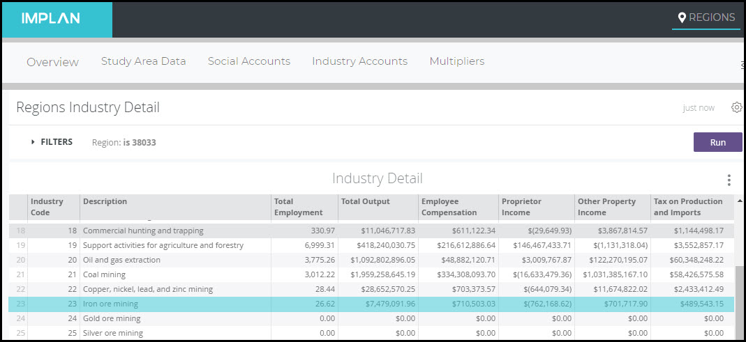
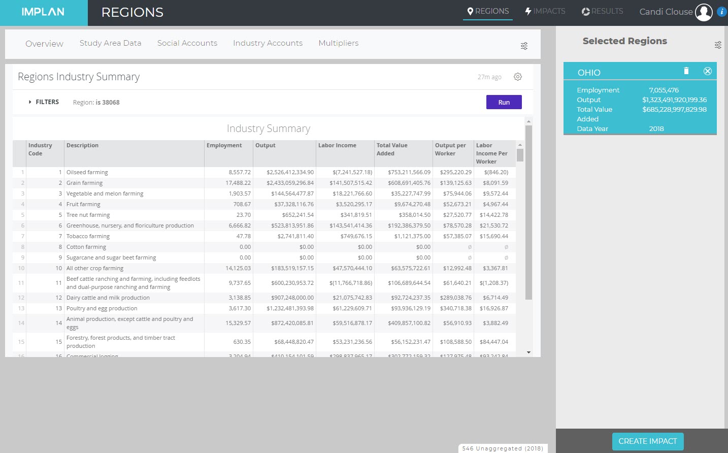
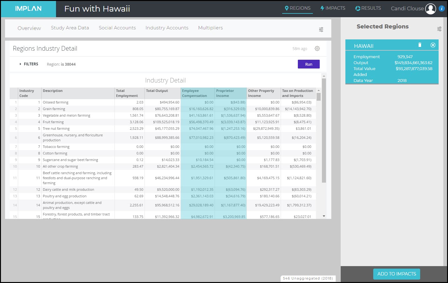
If you are looking for LQs for Employment, Labor Income, or Output, they are very easy to calculate using IMPLAN data. Select your Region and head Behind the i. On the Regions Overview screen the table at the bottom will list IMPLAN Industries with their associated Employment, Labor Income, and Output. You can download the table by clicking on the ellipses as shown. This will open up an Excel spreadsheet with the values.

You can use the LQ Template to calculate the Employment LQ for your Region against the U.S. Copy the Employment for all IMPLAN Industries from your downloaded file and paste them into Column E – Your Region’s Employment. The spreadsheet will automatically calculate the LQ in column G.

If you want to examine either Labor Income or Output, simply replace the national figures in Column C with the values for Labor Income or Output for the U.S. Then paste the Labor Income or Output value for your Region in Column E.

You can also compare your Region to something other than the nation. For example, we could look at the Charlotte–Concord–Gastonia Metropolitan Statistical Area compared to the state of North Carolina. In this case, simply replace Column C with the North Carolina values and Column E with the MSA values.

LQ Template

THE MATH

The formula is LQ =
Local Concentration / National (or reference Region) Concentration

More specifically the formula for the Employment LQ is:

LQ ir = (xir/xr) / (xin/xn)

where

xir = employment of sector i in region r

xr = total employment in region r

xin = employment of sector i in the reference region

xn = employment in the reference region

GOVERNMENT RESOURCES

BEA: What are location quotients (LQs)?

QCEW Location Quotient Details

REFERENCES

Bogart, W.T. (1998). The Economics of Cities and Suburbs. Upper Saddle River, NJ: Prentice Hall.

Grodach, C. & Ehrenfeucht, R. (2016). Urban Revitalization: Remaking Cities in a Changing World. New York: Routledge.

Wage & Salary Income

August 12, 2020/0 Comments/in Data Sources & Methodology, Glossary, Knowledge Base/by Joe Demski

Wage & Salary income includes base salary and/or wages, employee paid social insurance tax, bonuses, stock options, severance pay, profit distributions, and reimbursements for meals and lodging. It is a portion of Employee Compensation.

Location Quotient

August 12, 2020/0 Comments/in Glossary, Knowledge Base, Support Site/by Joe Demski

Location quotients (LQ) compare the relative concentration in a specific area to the concentration in the U.S. They are mainly used for descriptive and comparative purposes. The formula is LQ = Local Concentration / National Concentration, or more specifically the formula for the Employment LQ is:

LQ ir = (xir/xr) / (xin/xn)

where
xir = employment of sector i in region r
xr = total employment in region r
xin = employment of sector i in the reference region
xn = employment in the reference region

Typically, the reference region is the country in which region r resides, but it might also be a state or regional level. LQs can also be calculated using Output or Labor Income instead of Employment.

An LQ equal to 1 signifies that the local share is equal to the national share. An LQ of less than 1 means that the local share is less than the national share. An LQ of greater than 1 means the local share is greater than the national share and is typically an exporter or perhaps has a specialization in that Industry.

For more information, visit the BLS.

Categorizing Effects: Adding Back the Direct & Including Institutional Spending

August 12, 2020/0 Comments/in Knowledge Base, Output and Its Components, Support Site/by Joe Demski

INTRODUCTION

There are three possible types of Effects included in the Results of each analysis performed in IMPLAN: Direct, Indirect, and Induced. Direct Effects are the initial Final Demand Effect. Indirect Effects are generated due to demands from the regional supply chain to produce the final goods & services in the analysis, while Induced Effects are generated due to demands from households whose income is earned directly or indirectly due to their job activity in production being analyzed.

EFFECTS BY EVENT TYPE

Events that are designed to analyze Final Demand including Industry Events (Output, Employment, Employee Compensation and Proprietor Income), Industry Contribution Events, Commodity Output Events, and Institutional Spending Pattern Events. These will each have a Direct, Indirect, and Induced Effect. As shown in the table below this is not the case with all Event Types.

Direct, Indirect, & Induced	Indirect & Induced Only	Induced Only
Industry Events	Industry Spending Pattern Events	Labor Income Events
Industry Contribution Events		Household Income Events
Commodity Output Events
Institutional Spending Pattern Events

Industry Spending Pattern Events are designed to analyze effects due to the regional supply chain of the specified Industry. Industry Spending Patterns are made up of the Intermediate Inputs for the Industry and produce only Indirect and Induced Effects. Labor Income and Household Income Events are only designed to capture effects due to income earned in the analysis, producing Induced Effects only. Because Industry Spending Patterns Events and the two Income Events do not specify the exogenous change in Final Demand, these Event Types will not have a Direct Effect.

These categorization of Effects by Event Type are by design in IMPLAN and cannot be adjusted internally in the IMPLAN application. That being said, there are cases where it is appropriate to add in the “missing” Direct Effect or recategorizing Effects in the Results produced in IMPLAN.

DOWNLOAD RESULTS IN EXCEL

If manipulation of your Results is appropriate, start by downloading the results in the Results screen for whichever table you’d like to report. According to the following scenarios, adjust your Results accordingly. Remember to make the corresponding changes made in the Summary Results to any other Results tables you’ll be reporting.

RECATEGORIZING EFFECTS

ANALYSIS-BY-PARTS: INDUSTRY SPENDING PATTERN

Analyzing an Industry using Analysis-by-Parts is a workaround for the customization limitations in a single Industry Event. For this reason, the Results are not as straightforward as the Results produced in an Industry Event. When using an Industry Spending Pattern in your ABP, there will be only Indirect and Induced Effects. According to the IMPLAN Results, there is no Direct Effect, but adding in the known Direct Effect can be important for communicating the Total Effects of your analysis. If you’ve completed an ABP, you already have information on the Direct Labor Income, which should be included in the calculation of Direct Value Added and Direct Output. For an ABP you also must know either Direct Output or Direct Intermediate Inputs. Remember how Output breaks down:

If not all the Direct factors are known, estimates of these factors can be made from the underlying Study Area Data using the information found in:

Behind the i

> Customize Region

> Filter for Industry

You will find Output value ratios for the Industry you want to use. If the Industry does not exist in the Region, the Proxy region information must be used. Employment can be estimated using the Output per Worker ratios that are provided in:

Behind the i

> Study Area Data

> Industry Averages

The Direct Effect you produce should replace the effects of all zeros in the downloaded Excel format Results. The existing Indirect and Induced Effects are correct as is. The added Direct Effects can be summed with the existing Indirect and Induced Effects by column to produce the accurate Total Effects.

ANALYSIS-BY-PARTS: BILL OF GOODS APPROACH

When applying the Analysis-by-Parts technique using the Bill of Goods (BOG) Approach you are using a series of Commodity and/or Industry Effects instead of an Industry Spending Pattern. In the Results, your Direct Effects are from the Commodity/Industry Events, which actually reflect the Intermediate Input purchases made by the true Direct business. The Results should be modified such that these Direct Effects are reclassified as Indirect Effects. Once this step is completed, you should have only Indirect and Induced Effects, similar to the results when using an Industry Spending Pattern in an ABP as shown above. You can then add in the true Direct Effect as described in the previous section. Don’t forget to sum a new Total Effect.

Remember, if you’ve completed an ABP, you already have information on the Direct Labor Income, which should be included in the calculation of Direct Value Added and Direct Output. In this ABP approach, you also have information on the Direct Intermediate Inputs, which were analyzed as Commodity Events. If you’ve analyzed Commodity Output values that equal the total spending on each Commodity (locally and non-locally) by the Direct business, then the sum of Commodity Output values in all Commodity Output Events is equal to Direct Intermediate Inputs and can be summed with Direct Value Added to produce Direct Output.

If you are using this analysis approach because the Industry you are analyzing is not an Industry in the IMPLAN Industry Scheme and you are missing information about the Direct Effect, we recommend basing the Direct Effect calculations on the Industry that is most similar to the Industry you are analyzing with the BOG Approach.

INTERNALIZING OTHER INSTITUTIONAL EFFECTS

When analyzing Events in a single Region in IMPLAN, the application will generate effects due to spending by only one Institution: Households (in a Multi-Regional analysis trade “spending” is also internalized). Revenue for other Institutions can also be affected. For example, the Tax tab of your Results displays all the fiscal revenue supported by your analysis, but there will be no Direct, Indirect, or Induced Effects due the estimated tax collection being spent by the different levels of government.

Additional Events can be analyzed to produce these effects if enough information is known on how the Institution’s spending will be affected. In any analysis that includes Institution spending of revenue derived from an already present Direct Effect, you should treat all effects of that spending as Induced. Direct, Indirect, and Induced Effects should be summed and recategorized as Induced Effects when using an Institutional Spending Pattern or any other Event Type to manually internalize the effects of secondary demands from Insitutitions (other than Households) expected to be supported by the other Events being analyzed.

These Induced Institutional Effects can be combined with the original Effects produced by the Event. In which case a new Total Effect would need to be calculated.

Local Industries Buying Local

August 12, 2020/0 Comments/in Margins, Local Purchase Percentages and Deflators, Support Site/by Joe Demski

INTRODUCTION

Did you ever wonder how much local bread your local supermarkets buy? Or how much local auto manufacturers spend on local tires? The process to find this answer may seem complicated, but it is actually relatively simple. Here’s how.

THE PROCESS

Let’s examine how much local beer is purchased by local restaurants in Greater Milwaukee. Start by selecting your Region (Milwaukee-Waukesha, WI MSA 2018 shown below) and heading into the data for Commodity 3106 – Beer, ale, malt liquor and nonalcoholic beer.

STEP 1: FIND THE TOTAL COMMODITY SUPPLY

Behind the i

> Social Accounts

> Reports

> Commodity Summary

> Total Commodity Supply

The Total Commodity Supply for beer is $672,638,420.90. This represents the total beer supply produced in Milwaukee by both Industries and Institutions.

STEP 2: FIND THE REGIONAL INPUTS

Behind the i

> Social Accounts

> Balance Sheets

> Industry Balance Sheet

> Commodity Demand

> Filter for Industry 509 – Full-service restaurants

> Regional Inputs

Scroll to Commodity 3106 – Beer, ale, malt liquor and nonalcoholic beer and find the value for Regional Inputs. For the Milwaukee-Waukesha, WI MSA this is $4,196,438.53. Regional Inputs show the amount that restaurants spend locally on beer during the Data Year. Note that the Gross Inputs of $11,686,495.43 represent the total annual spending on beer by full-service restaurants. We then know that local restaurants are spending 35.91% of their beer budget on local brews (RPC = 35.91%).

STEP 3: DIVIDE THE RESULTS

The Regional Inputs of $4M divided by the Total Commodity Supply of $673M tell us that Milwaukee restaurants are buying less than 1% of total local beer production. Given how much beer production occurs in the Region, the percentage of local beer production that is purchased by local restaurants is quite low. The table below compares four cities on the percentage that local restaurants spend on local beer.

STEP 4: EXAMINE EXPORTS

Behind the i

> Social Accounts

> Reports

> Commodity Trade

Now we can look at exports. Foreign Exports tells us the total local production that is exported outside the U.S. The Domestic Exports tells us the total local production that leaves Greater Milwaukee but stays in the U.S. The Total Exports is a combination of these two. The Total Exports from Milwaukee is $583,403,228.86. Taking this divided by the Total Commodity Supply of $672,638,420.90 tells us that 87% of the locally produced beer is exported from the MSA. Therefore, 13% stays local – which is known as the Average RSC (Regional Supply Coefficient).

STEP 5: INCREASE LOCAL BEER PURCHASES

Let’s say local restaurants want to commit to purchasing a full 50% of their beer from local breweries. They are currently spending a total of $11,686,495.43 on beer, so half would be $5,843,247.72. They are currently spending $4,196,438.53, so they would need to increase their local buy by $1,646,809.19. We can run this as an Industry Output Event.

The Results show us that the increase in $1,646,809.19 in local breweries supports a total Output of $2,514,260.11; a multiplier of 1.53. This will support almost 3 employees at the brewery and 4 additional employees in the Indirect and Induced Effects; a multiplier of 2.53.

Negative Multipliers

August 12, 2020/0 Comments/in Support Site, Understanding the Model/by Joe Demski

INTRODUCTION

Multipliers measure the economic change within a Region that stems from economic activity from a change in Final Demand. They are a measure of an Industry’s connection to the wider local economy by way of input purchases, payments of wages and taxes, and other transactions. They are the total production impact within the Region for every unit of direct production.

There are two main types of multipliers. For more details, check out the article Understanding Multipliers.

Type I Multiplier = (Direct Effect + Indirect Effect) / (Direct Effect)

Type SAM Multiplier = (Direct Effect + Indirect Effect + Induced Effect) / (Direct Effect)

And yes, sometimes they are negative. Here are the details.

DETAILS

Let’s take a look at an example. In Alabama 2018 Industry 23 – Iron Ore Mining, there is negative Proprietor Income.

Behind the i

> Region Details

> Study Area Data

> Industry Detail

Negative_Mulitpliers_-_AL_Iron_Ore_Mining_Negative_PI.jpg

So we know that there was a net loss for Proprietor Income in 2018 in this Industry. Proprietors could have lost money or spent more money from savings than they earned. This doesn’t mean that they went out of business. They could be just using savings or borrowing money to maintain their cash flow. For further details on why this happened, read the article The Curious Case of the Negative Tax: Agriculture Subsidies, Profit Losses, and Government Assistance Programs.

Labor Income is equal to Proprietor Income + Employee Compensation. Because we saw a negative in Proprietor Income that was larger than the positive Employee Compensation, there is negative Labor Income in this Industry. When we analyze increased production in this industry, IMPLAN estimates negative Direct Labor Income. When an Industry has this negative relationship between Output and Labor Income, the total Labor Income supported by increased production is typically positive while the Direct Labor Income is negative. This produces a negative Labor Income Multiplier.

Behind the i

> Multipliers

> Summary Multipliers

> Labor Income Multipliers

Negative_Mulitpliers_-_AL_Iron_Ore_Mining_Negative_LI_Mult.jpg

In a bad year (low prices or spikes in operational costs), an Industry can lose money. Losses in any piece of Value Added (Employee Compensation, Proprietor Income, Taxes on Production & Imports, or Other Property Income) can create a negative multiplier if those losses aren’t offset by larger gains in another piece of Value Added. For example, in IMPLAN, the combination of Proprietor Income and Other Property Income equals operating surplus. The operating surplus of an Industry is simply its profits – that is, value of production minus all operational expenditures. If the negative operating surplus exceeds Employee Compensation plus Taxes on Production & Imports, then total Value Added will be negative. Industries with a negative relationship between Output and Value Added usually have a negative Value Added Multiplier, like in the case of Labor Income.

Economic Impact Reporter’s Toolkit

August 12, 2020/0 Comments/in Knowledge Base, Support Site/by Joe Demski

Understanding Intermediate Inputs (II)

February 27, 2020/0 Comments/in Knowledge Base, Output and Its Components, Support Site/by Joe Demski

INTRODUCTION:

Let’s get this out of the way right off the bat. Intermediate Inputs were previously called Intermediate Expenditures in IMPLAN. Much like Prince (once known as only a Love Symbol) or Sean (middle name now “Love” not “Diddy”) Combs, sometimes we have to change names. And you will love this one!

We changed the title to be consistent with the definition and terminology of the Bureau of Economic Analysis (BEA). The BEA defines Intermediate Inputs as “Goods and services that are used in the production process of other goods and services and are not sold in final-demand markets.”

Intermediate Inputs are purchases of non-durable goods and services such as energy, materials, and purchased services that are used for the production of other goods and services, rather than for final consumption. They do not include any capital-account purchases or labor.

DETAILS:

The first round of Indirect Effects are triggered by the Intermediate Inputs purchased by the Direct business or businesses when analyzing Industry Events, Commodity Events, Industry Contribution Events, and Institutional Spending Pattern Events. The amount of Intermediate Inputs is solely determined by the Event’s Direct Output and the relationship between Output and Intermediate Inputs according to the Direct Industry’s Total Gross Absorption. Further rounds of Indirect Effects reflect the ripple effect through the local Supply Chain. The local businesses affected in the first round of Indirect Effects also purchase Intermediate Inputs from local businesses, and so on.

Labor Income and Household Income Events do not generate any Indirect Effects but there are Intermediate Inputs still being analyzed in them. In these Events the income spent at local businesses is being estimated and analyzed. The Intermediate Inputs of the Inducedly affected business triggers further rounds of Induced Effects.

When using an Industry Spending Pattern Event the first round of Indirect Effects are triggered by the Intermediate Inputs being analyzed. The amount of Intermediate Inputs is solely determined either by the Event Value alone (by default Industry Spending Pattern Event Values are total Intermediate Inputs) or by the relationship between Output and Intermediate Inputs according to the specified Industry’s Total Gross Absorption when “Total Output” is selected in the Advanced Menu of the Event instead of Intermediate Inputs.

Industry Spending Pattern Events are appropriate when modifications to the Intermediate Inputs of an Industry’s Leontief Production Function are necessary. When detailed information is known about Intermediate Input spending, these Events can be used and adjusted to reflect the specific purchases or ratios of purchases. Industry Spending Patterns include all Intermediate Inputs for a given Industry.

Institutional Spending Patterns are unique in that they describe both Intermediate Inputs and Value Added within the same Spending Pattern. The Results in Institutional Spending Patterns differ: the reported Direct Effects describe both what we would generally consider Direct Effects (income, Employment and Value Added) and the first-round Indirect Effects that arise from the government spending its budget.

WHERE TO FIND IT IN IMPLAN:

ON THE REGIONS SCREEN

Intermediate Inputs represent the difference between Output and Value Added. To calculate Intermediate Inputs, head to the table Behind the i called Regions Industry Summary by navigating to

> Study Area Data

> Industry Summary

If we look at Industry 1 – Oilseed farming in Ohio for example, we can calculate Intermediate Inputs

= Output – Total Value Added

= $2,526,412,335 – $753,211,566.09

= $1,773,200,769

ON THE IMPACTS SCREEN

On the Impacts screen, you can see the Spending Pattern for Industries by choosing the Industry Spending Pattern Event Type or for Institutions by choosing the Institutional Spending Pattern Event Type. By clicking on the menu icon and choosing Advanced, you can see the list of Commodities purchased as inputs by that Industry or Institution.

ON THE RESULTS SCREEN

The Summary Results has a table entitled Economic Indicators by Impact. To calculate the Intermediate Inputs, simply take Output less Value Added. Therefore in this example, Intermediate Inputs

= Output – VA

= $829,827 – $392,848

= $436,979

HOW IS IT CALCULATED?

IMPLAN defines Intermediate Inputs as:

Or more simply,

So to calculate Intermediate Inputs, we just take Output less the other four components of the Leontief Production Function (which sum to Valued Added).

Intermediate Inputs

February 27, 2020/0 Comments/in Glossary, Knowledge Base, Support Site/by Joe Demski

Goods and services that are used in the production process of other goods and services and are not sold in final-demand markets (BEA). Intermediate Inputs consist of purchases of non-durable goods and services such as energy, materials, and purchased services that are used for the production of other goods and services rather than for final consumption. They do not include any capital-account purchases nor do they include the inputs from the primary factors of production (capital and labor) that are components of value added.

These inputs are sometimes referred to as current-account expenditures. In IMPLAN, this was previously referred to as Intermediate Expenditures.

Understanding Labor Income (LI), Employee Compensation (EC), and Proprietor Income (PI)

February 21, 2020/0 Comments/in Knowledge Base, Support Site/by Joe Demski

INTRODUCTION:

Labor Income is the sum of Employee Compensation (wages and benefits) and Proprietor Income. Labor Income represents the total value of all forms of employment income paid throughout a defined economy during a specified period of time. It reflects the combined cost of total payroll paid to employees (e.g. wages and salaries, benefits, payroll taxes) and payments received by self-employed individuals and/or unincorporated business owners (e.g. capital consumption allowance) across the defined economy.

DETAILS:

Labor Income consists of two parts. The first, Employee Compensation, is the total payroll cost of wage and salary employees to the employer. This includes wages and salaries, all benefits (e.g., health, retirement) and payroll taxes (both sides of social security, unemployment insurance taxes, etc.). It is also referred to as fully-loaded payroll.

The second piece of Labor Income is Proprietor Income (PI). PI consists of payments received by self-employed individuals and unincorporated business owners. More specifically, it represents the current-production income of sole proprietorships, partnerships, and tax-exempt cooperatives. It includes the capital consumption allowance and is recorded on Federal Tax form 1040C. It excludes dividends, monetary interest received by nonfinancial business, and rental income received by persons not primarily engaged in the real estate business.

Note that IMPLAN’s estimated Employee Compensation and Proprietor Income fields represent the average payroll values for all employees that work in a firm, across all Industries that report in the Study Area’s region.

Labor Income generates Induced Effects via the spending by local residents that are employed by the direct business or businesses. The local residents employed by the Indirect businesses also generate Induced Effects due to their spending. If no Labor Income is entered into the Event, IMPLAN will calculate it by the ratio of the Industry’s Labor Income to Output. Note, if Labor Income information is entered in your Event in addition to Output, IMPLAN will not re-balance Output.

WHERE TO FIND IT IN IMPLAN:

Labor Income can be found in IMPLAN Behind the “i” in the Study Area Data tab. Within the Industry Detail table you will find the two forms of Labor Income, Employee Compensation and Proprietor Income, by Industry. Within the Industry Summary table you will find Labor Income as a total and Labor Income per Worker by Industry.