Multipliers measure the economic change within a Region that stems from economic activity from a change in Final Demand. They are a measure of an Industry’s connection to the wider local economy by way of input purchases, payments of wages and taxes, and other transactions. They are the total production impact within the Region for every unit of direct production.
There are two main types of multipliers. For more details, check out the article Understanding Multipliers.
Type I Multiplier = (Direct Effect + Indirect Effect) / (Direct Effect)
Type SAM Multiplier = (Direct Effect + Indirect Effect + Induced Effect) / (Direct Effect)
And yes, sometimes they are negative. Here are the details.
DETAILS
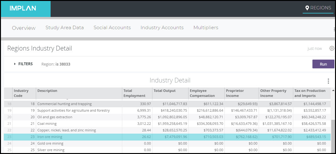
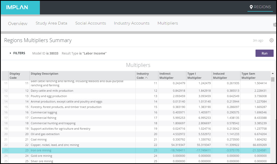
Let’s take a look at an example. In Alabama 2018 Industry 23 – Iron Ore Mining, there is negative Proprietor Income.
So we know that there was a net loss for Proprietor Income in 2018 in this Industry. Proprietors could have lost money or spent more money from savings than they earned. This doesn’t mean that they went out of business. They could be just using savings or borrowing money to maintain their cash flow. For further details on why this happened, read the article The Curious Case of the Negative Tax: Agriculture Subsidies, Profit Losses, and Government Assistance Programs.
Labor Income is equal to Proprietor Income + Employee Compensation. Because we saw a negative in Proprietor Income that was larger than the positive Employee Compensation, there is negative Labor Income in this Industry. When we analyze increased production in this industry, IMPLAN estimates negative Direct Labor Income. When an Industry has this negative relationship between Output and Labor Income, the total Labor Income supported by increased production is typically positive while the Direct Labor Income is negative. This produces a negative Labor Income Multiplier.
In a bad year (low prices or spikes in operational costs), an Industry can lose money. Losses in any piece of Value Added (Employee Compensation, Proprietor Income, Taxes on Production & Imports, or Other Property Income) can create a negative multiplier if those losses aren’t offset by larger gains in another piece of Value Added. For example, in IMPLAN, the combination of Proprietor Income and Other Property Income equals operating surplus. The operating surplus of an Industry is simply its profits – that is, value of production minus all operational expenditures. If the negative operating surplus exceeds Employee Compensation plus Taxes on Production & Imports, then total Value Added will be negative. Industries with a negative relationship between Output and Value Added usually have a negative Value Added Multiplier, like in the case of Labor Income.
In IMPLAN, there are four types of income that can be identified: Labor Income, household income, disposable income, and household spending. This article breaks down the differences and how IMPLAN data compares to government estimates.
DEFINING INCOME:
First off, let’s define the fours types of income.
LABOR INCOME
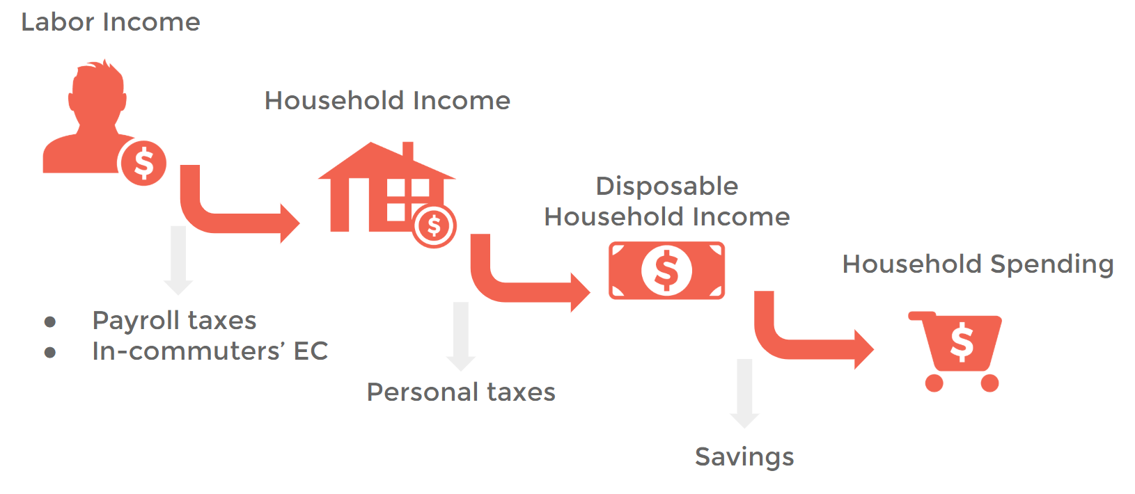
Labor Income is the sum of Employee Compensation (wages and benefits) and Proprietor Income.
HOUSEHOLD INCOME
Household income represents the income from all sources received by residents, including total wages & salaries, benefits, interest, dividends, & transfer payments, less all contributions to Social Security/Medicare. Labor Income less payroll taxes and in-commuting income is included in household income in addition to all non-employment sources of household income. This is based on the BEA definition of personal income and is not comparable to money income as defined by the Census Bureau.
DISPOSABLE HOUSEHOLD INCOME
Disposable income is household income less personal taxes. Disposable Income is money that is available to be saved or spent.
HOUSEHOLD SPENDING
Household spending is what is actually expended by households on goods and services less personal taxes and savings.
WHERE TO FIND THEM IN IMPLAN:
LABOR INCOME
Labor Income can be found in IMPLAN Behind the “i” in the Study Area Data tab. Within the Industry Detail table you will find the two forms of Labor Income, Employee Compensation and Proprietor Income, by Industry. Within the Industry Summary table you will find Labor Income as a total and Labor Income per Worker by Industry.
In the Social Accounting Matrix (SAM) you will find Employee Compensation and Proprietor Income represented as columns and rows. The columns reflect the allocation of each of these forms of income to each row, largely to Households. The rows reflect all sources of Employee Compensation and Proprietor Income. Because Labor Income is only earned from Industries, you’ll only find a value in the Industry column of these rows.
HOUSEHOLD INCOME
Household Income can be calculated as the sum of all nine Household Income column totals from the Social Accounting Matrix. Each Household Income row here shows all the sources of Household Income, which in large part will be Labor Income.
DISPOSABLE HOUSEHOLD INCOME
Disposable Household Income can be calculated as Household Income as described above less the payments to government rows within the Household Income columns.
HOUSEHOLD SPENDING
Household Spending can be calculated as the sum of payments to the Commodity total row and Foreign and Domestic Trade rows within each Household Income column in Aggregate SAM. These payments reflect Household Spending on goods and services sourced from within the Region (payments to Commodity row) and outside of the Region (payments to trade rows).
UNDERSTANDING THEIR RELATIONSHIP:
TWO EVENT TYPES:
To model spending of individuals, there are two Event Types in IMPLAN.
LABOR INCOME EVENTS
Labor Income Events are most appropriate to use when an analyst intends to model a change in labor payments isolated from an industry’s production. When creating a Labor Income Event in IMPLAN, analysts may specify whether the income is earned by employees (wage and salary), by proprietors, or some combination of the two. However, they cannot specify the specific household income categories which will receive that income.
Labor Income Event Value should include all new labor payments in the Region (local workers and in-commuters), including their
Payroll tax
Personal tax
Savings
HOUSEHOLD INCOME EVENTS
Household Income Events are most appropriate to use when an analyst intends to model changes in household income that are independent of both production and payroll. In Household Income Events (unlike Labor Income Events), you can specify the specific income group(s) receiving the income into one of nine categories.
Household Income Event Values should include all new household income all residents in the region, including their –
Personal tax
Savings
USING WAGE & SALARY INCOME DATA
When you’d like to analyze wage and salary income data, it must be first converted into a fully loaded Employee Compensation value before entering the value into your Labor Income Event. Employee Compensation in IMPLAN is the fully loaded cost of the employee to the employer, therefore a wage and salary value would be missing the employer’s cost of benefits and contribution to Social Insurance Tax.
You can use the following resource to convert your wage and salary income to an Employee Compensation value as well as to convert an Employee Compensation value in the IMPLAN data or Results to a wage and salary income value.
USING DISPOSABLE INCOME OR HOUSEHOLD SPENDING DATA
If you’d like to analyze a change in disposable income, you can adjust a disposable income value to a household income value by dividing your disposable income value by the portion of household income (for a given income group column) allocated to non-government rows. In other words, dividing household income by the portion of household income that is disposable income for a given household income group. This will produce a value that can be entered in a Household Income Event. Similarly, dividing household spending by the portion of household income that is for household spending will produce a value that can be entered in a Household Income Event.
CONSIDERATIONS FOR USING AN INCOME EVENT:
Labor Income Events are commonly and appropriately used for analyzing the impact of wage increases and business operations where Analysis-by-Parts is needed such that Labor Income and Industry Spending on goods and services are analyzed as two separate Events.
Household Income Events are commonly and appropriately used for analyzing new income in a Region due to new residents that live in the Region but do not work there.
Households and individuals may experience other economic shocks that increase or decrease the amount of income available to them. Before analyzing any impacts in IMPLAN its important to consider the underlying assumptions and then state the assumptions made in your analysis when reporting the results.
For example, if a policy change results in savings to households due to a reduction in cost on necessary goods and services such as electricity or insurance, how might these households react? If this household is living paycheck to paycheck, they may spend this newly available income on the items they typically buy. If so, a household income event would be appropriate. If this household already has their expenses covered maybe they go out to the movies more often, maybe they buy a few things on Amazon, or maybe they save it up for a future purchase like a new car. In this case a Household Income Event would not be appropriate since this household would not be appropriate. These considerations are explored further, specifically in the context of Utility Purchases and Energy Rebates here.
ONE MAJOR SOURCE OF CONFUSION:
So, you may look at the data Behind the i and then get ready to email your Customer Success Manager at support@implan.com to announce that what IMPLAN is reporting for Household Income is not even close to what the Census Bureau reports for Household Income. It’s OK, we know.
IMPLAN uses the BEA’s definition, which is not the same as what the Census uses. So, you won’t be able to compare these two sources. For more information on this, check out our article Why is Personal Income for My Region so High? Basically, the BEA definition includes imputed income, adjustments for misreporting and under-reporting, and employment paid benefits.
https://implan.com/wp-content/uploads/Market-site-Logo-resized-2-1.jpg00Joe Demskihttps://implan.com/wp-content/uploads/Market-site-Logo-resized-2-1.jpgJoe Demski2020-02-21 14:06:482020-02-21 14:07:16Understanding Types of Income
Dollar Year is the year represented by the values in your Event. This is usually (but not always) the same as the year in which your event occurred or is expected to occur.
IMPACTS SCREEN
On the Impacts screen, Dollar Year should be the year of the data you are inputting.
RESULTS SCREEN
On the Results screen, Dollar Year shows the year of the value of the economic indicators – the year of what you want your results to show.
For an example of when Dollar Year on the Impacts screen will not be the year in which you event occurred, suppose you were borrowing a visitor expenditure pattern from a survey that was done in 2015. But let’s say you want to use this data to estimate visitor spending in 2020. In this case, while the year of your event (that is, the year of the visits) is 2020, those dollars still represent 2015 dollars and must be characterized as such in order to generate correct results. By correctly telling IMPLAN that those values are 2015 values (by setting Dollar Year to 2015 on the Impacts screen), IMPLAN will know to inflate those values to the Data Year to ensure the correct values are applied to the multipliers.
If you are setting up your event with an employment value instead of a dollar value (only recommended if you do not have a dollar value with which to start the set-up of your Event), Dollar Year should be set to the year in which that employment took place or is expected to take place.
Defining Dollar Year in the Impacts screen correctly is essential to getting accurate Results. On the other hand, how Dollar Year is defined in the Results screen is totally up to you and how you want to report your Results. If we want to report the effect of our 2020 visitors is 2020 dollars, we simply need to ensure the Dollar Year in the Results screen is filtered to 2020. Dollar Year in the Results screen will default to the current year. Remember, dollars can only be summed or compared when in like Dollar Years.
DATA YEAR:
Data Year is the year of the dataset that you are utilizing. Currently, IMPLAN has datasets for 2001-2018. We recommend using the Data Year that matches your data, the year your Events took place. If you are modeling something that occurred in the current year or is expected to happen in the future, we recommend using the most current dataset, 2018.
The Regions screen will show you data from 2001-2018 in the 546 Industry Scheme. To access datasets in the 536 Industry Scheme, start your analysis from the Projects screen and click New Project in the upper right.
FOR 2012 – 2014 DATA YEARS IN THE 536 INDUSTRY SCHEME
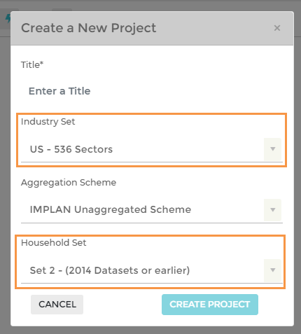
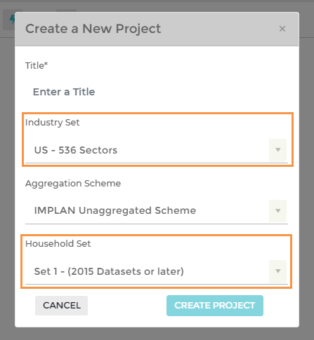
Give your project a name and then under Industry Set choose US – 536 Sectors and Household Set choose Set 2 – 2014 Datasets or earlier. Once you’ve created the Project you will have access to the datasets from 2012-2014 (in the 536 Industry Scheme) in the drop-down menu at the top of the Regions screen (where you will be automatically redirected).
FOR 2015 – 2017 DATA YEARS IN THE 536 INDUSTRY SCHEME
Give your project a name and then under Industry Set choose US – 536 Sectors and Household Set choose Set 1 – 2015 Datasets or later. Once you’ve created the Project you will have access to the datasets from 2015-2017 (in the 536 Industry Scheme) in the drop-down menu at the top of the Regions screen (where you will be automatically redirected).
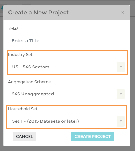
FOR 2018 DATA YEAR IN THE 546 INDUSTRY SCHEME
Give your project a name and then under Industry Set choose US – 546 Sectors and Household Set choose Set 1 – 2015 Datasets or later. This will give you access to the 2018 dataset, which is only available in the 546 Industry Scheme.
https://implan.com/wp-content/uploads/Market-site-Logo-resized-2-1.jpg00Joe Demskihttps://implan.com/wp-content/uploads/Market-site-Logo-resized-2-1.jpgJoe Demski2019-12-09 14:52:042020-08-14 13:12:58Dollar Year & Data Year
So you ran your Industry Event impact and you get to the Results screen. Great! But have you ever wondered exactly what each of those boxes in your summary results mean? This is the article for you!
There are nuances with each type of Event you run. This article specifically addresses the Industry Output, Industry Employment, Industry Employee Compensation, and Industry Proprietor Income Event types.
INTERPRETING THE RESULTS:
Let’s walk through an example. Andrew’s Bootleg, a craft vodka company, went legit in 2019. We modeled his $1.5M in Output on the state of North Carolina. Our results are as follows:
Now let’s unpack exactly what his sales mean for the North Carolina economy. We see a total impact of 4.3 jobs, $471,347 in Labor Income, $1.4M in Value Added, and $2.0M in Output. This is the total economic impact from Andrew’s Bootleg; the sum of the Direct, Indirect, and Induced effects. Each of the next sections outlines what each part of this impact actually means.
EMPLOYMENT:
DIRECT EMPLOYMENT
The 0.95 Direct Employment show that with $1.5M in Direct Output, it looks like Andrew can almost support himself full-time. This figure is the direct number of job years associated with the Output. But remember, jobs in IMPLAN are average annual employment. To switch between IMPLAN jobs and FTE, use the 536 FTE & Employee Compensation Conversion Table (2017). Using this converter, we see that the 0.95 IMPLAN jobs translate to .91 FTE jobs.
INDIRECT EMPLOYMENT
Andrew has to buy things like corn and yeast for his distilling. Because he is able to purchase some of his inputs from within the state, 1.19 jobs are supported in business-to-business transactions with the corn and yeast (and other) suppliers, as well as suppliers of those suppliers in the state. This Indirect employment represents the number of job years that are supported by business to business transactions as a result of the economic activity generated by the Event.
INDUCED EMPLOYMENT
Andrew himself, and the employees in the businesses supported by Andrew’s operational purchases, spend a lot of their take-home income in North Carolina on things like paying rent and buying groceries. Through this, 2.16 jobs are supported in industries like real estate, health care and restaurants. Induced employment represents the number of job years that could potentially be supported by household spending as a result of the economic activity generated by the Event.
LABOR INCOME:
DIRECT LABOR INCOME
Andrew pays himself well. The $292,512 in Direct Labor Income is the sum of the Employee Compensation (EC) and Proprietor Income (PI) paid to that one (0.95) employee. Even though EC includes wages and salaries, all benefits (e.g., health, retirement), and payroll taxes, he still takes home quite a bit. To switch between IMPLAN Employee Compensation and Wage & Salary figures, we can again use the 536 FTE & Employee Compensation Conversion Table (2017). Using this converter, we estimate that Andrew will take home $236,276 in wages. Direct Labor Income is the initial income earned by the Direct employees of the Industry specified in the Event.
INDIRECT LABOR INCOME
The $83,289 in Indirect Labor Income is the EC and PI that Andrew’s Bootleg supports in the corn and yeast (and other) suppliers. Indirect Labor Income is the amount of EC and PI that is associated with business-to-business transactions as a result of the economic activity generated by the Event.
INDUCED LABOR INCOME
Because Andrew and the other supported workers are spending their paychecks around the state, there is an Induced Labor Income of $95,546, including both EC and PI. Induced Labor Income is the amount of EC and PI that is associated with household spending as a result of the economic activity generated by the Event.
VALUE ADDED:
DIRECT VALUE ADDED
Value Added is akin to Gross Domestic Product (GDP) or at the North Carolina level, Gross State Product (GSP). Value Added includes the Labor Income dollars, as well as Taxes on Production and Imports (TOPI) and Other Property Income (OPI). Andrew’s Bootleg contributes $1.0M in Direct Value Added. Remember, this includes the $292,512 in Labor Income, plus TOPI plus OPI.
INDIRECT VALUE ADDED
Through the business-to-business transactions, the company contributes $131,417 to Value Added or GSP. Again, this includes the $83,289 in Indirect Labor Income plus TOPI plus OPI. This is the specific Value Added that is generated by business to business transactions as a result of the economic activity generated by the Event.
INDUCED VALUE ADDED
Because of the spending of the employee working at Andrew’s Bootleg and the supply chain companies, $175,477 of Value Added is supported. This includes the $95,546 of Induced Labor Income, plus TOPI plus OPI. This is the specific Value Added that is generated from household spending as a result of the economic activity generated by the Event.
OUTPUT:
DIRECT OUTPUT
Andrew’s Bootleg has a Direct Output of $1.5M. We know this because that’s what we modeled. Output is equal to Value Added plus Intermediate Expenditures; it is the total value of production. Remember, it includes Value Added (and Value Added includes Labor Income). Output is also the basis for all other calculations in IMPLAN. Total production value or Output, includes unsold production and excludes sold inventory. If Andrew sells all of his vodka produced this year within the year and only sells vodka produced this year, his $1.5M of Direct Output will be equivalent to his 2019 revenue.
INDIRECT OUTPUT
Because of the business-to-business transactions resulting from local input purchases by Andrew’s Bootleg, $244,801 in Output is supported. Indirect Output represents all of the Output generated because of the Direct business to business spending. This figure includes the $131,417 in Indirect Value Added; and that Value Added then includes the $83,289 in Indirect Labor Income.
INDUCED OUTPUT
Finally, $304,130 of Induced Output is supported when the employees working at the distillery and their suppliers (and the suppliers of their suppliers) spend their money throughout the economy. Induced Output is the total value that all industries take in as a result of household spending. This figure includes the $175,477 in Induced Value Added; and that Value Added then includes the $95,546 in Induced Labor Income.
BOOTLEG BREAKDOWN:
And that’s it! You can use this guide to help you understand the individual effects of your IMPLAN analysis. I’ll drink to that!
https://implan.com/wp-content/uploads/Market-site-Logo-resized-2-1.jpg00Joe Demskihttps://implan.com/wp-content/uploads/Market-site-Logo-resized-2-1.jpgJoe Demski2019-12-09 14:35:412019-12-09 14:35:53What are Direct, Indirect, and Induced Impacts?
Multipliers are the basis of how an I-O Analysis System such as IMPLAN makes estimations of the potential impacts of economic changes. Expressed as a rate of change, a Multiplier describes how for a given change in a particular Industry a resultant change will occur in the overall economy (e.g. for every dollar spent in the economy an additional $0.25 of economic activity is generated locally, implying a Multiplier of 1.25).
This article describes what a Multiplier means, the basis of how we can determine that an additional $0.25 will occur locally, and introduces the idea of aggregating Industries if you are trying to find the impact across a broad spectrum of production rather than a specific Sector.
DETAILED INFORMATION:
Multipliers exist in the IMPLAN Model to describe rates of changes for several different variables. The descriptions below apply to Type SAM and Type I Multipliers, which are unitless values.
Output – Output is the base Multiplier from which all other Multipliers are derived. The Output Multiplier describes the total Output generated as a result of 1 dollar of Output in the target industry. Thus if an Output Multiplier is 2.25, that means that for every dollar of production in this Industry $2.25 of activity is generated in the local economy: the original dollar and an additional $1.25.
Employment – Employment Multipliers describe the total jobs generated as a result of 1 job in the target industry. Thus if an Employment Multiplier is 2.33, that means that every Direct Job creates 2.33 jobs in the total economy: the original job and 1.33 additional jobs.
Labor Income – Labor Income Multipliers describes the dollars of Labor Income generated as a result of one dollar of Labor Income in the target Industry. A Labor Income Multiplier of 2.2 indicates that for every dollar of Direct Labor Income in this Industry another $1.20 of Labor Income is generated in the local economy.
Value Added – Value Added Multipliers describe the total dollars of Value Added generated as a result of one dollar of Value Added in the target Industry. A Value Added Multiplier of 2.3 indicates that for every dollar of Direct Value Added in this Industry another $1.30 of Value Added is generated in the local economy.
You can also compare Sectors’ Multipliers across regions. You will find that Multipliers are generally larger the larger the Study Area is. This is the result of a typical pattern that describes that larger regions will have less leakage to imports. Thus for accurate comparisons, it is most appropriate to compare states to states and counties to counties.
TYPE I VS. TYPE SAM MULTIPLIERS:
Type I and Type SAM Multipliers differ in their definition of “total” impact
Type I – Looks only at business to business purchases and does not include the effects of local Household spending. This Multiplier is calculated as: (Direct + Indirect Effects) / Direct Effect.
Since the denominator for the multiplier is always 1.00, the Type I Multiplier will equal the Direct Effect + the Indirect Effect
Thus, the Type I Multiplier for Employment describes the direct and supply chain jobs within the study region resulting from one direct job.
Type SAM – In addition to the Type I Multiplier, the Type SAM Multiplier includes the impact of Household spending and is the more common Multiplier. It is calculated as: (Direct + Indirect + Induced Effects) / Direct Effect.
For example, the Type SAM Multiplier for Output describes the total output created in the study region resulting from one dollar of direct output.
It also includes other non-industrial transactions, such as institution savings, payment of social security taxes, and commuting.
EFFECTS VS. MULTIPLIERS:
When the dollars or jobs associated to all the rounds of local purchasing are summed, the resultant values are the Effects. The Multiplier Effects come in 4 types:
Direct Effect
For Output, these effects are either 1.00 or 0.00. For every dollar spent in an Industry, if the Industry exists in the region, there is a dollars worth of activity in the local economy. If the Industry doesn’t exist in the region, the effect is 0.00.
For Employment, the Effect represents the number of jobs per $1,000,000 of production in the Industry.
Labor Income Effects represent the Labor Income dollars per $1,000,000 of production in the Industry.
Value Added Effects represent the Total Value Added and various Value Added subset dollars per $1,000,000 of production in the Industry.
Indirect Effects
For Output, the Effect represents the sum of local business to business purchases per dollar of Output.
For Employment, the Effect represents the number of jobs per $1,000,000 of business to business purchases by all resultant rounds of local Industry purchases.
Labor Income Effect represents the value of Labor Income dollars per $1,000,000 of business to business purchases by all resultant rounds of local Industry purchases.
Value Added Effect represents the of Value Added dollars per $1,000,000 of business to business purchases by all resultant rounds of local Industry purchases.
Induced Effects
For Output, the Effect represents the sum of local Household purchases per dollar of Output, based on Labor Income payments made by the target Industry and the local Industries from which they purchase.
For Employment, the Effect represents the number of jobs supported in local Industries per $1,000,000 of Direct spending in the target Industry as a result of Household purchases derived from Labor Income payments throughout all rounds of the impact.
Labor Income Effect represents the value of Labor Income dollars per $1,000,000 of Direct spending in the target Industry in local Industries as a result of Household purchases derived from Labor Income payments throughout all rounds of the impact.
Value Added Effect represents the Value Added dollars per $1,000,000 of Direct spending in the target Industry in local Industries as a result of Household purchases derived from Labor Income payments throughout all rounds of the impact.
Total Effects are the sum of the Direct, Indirect, and Induced Effects. For Output, this value is the same as the SAM Multiplier.
HOW MULTIPLIERS ARE CREATED:
While the complex process of creating the Social Accounting Matrix is not described here, the results of those calculations are a complete transactions table showing what every Industry needs to purchase in order to make its products and the value of every Industry’s labor payments (Labor Income), taxes (Taxes on Production & Imports), and profits (Other Property Type Income) and what each Household income group buys.
We also know how much of each commodity is produced locally, which Industries or Institutions produce it in the local economy, and how much of the production is attributed to each producer.
The combination of these two factors allows the software to determine, based on the entered or estimated value of Industry Sales, how much of each commodity will be required to meet the change in production of the target Industry (Gross Absorption) and how much can be obtained from local vendors (Regional Absorption). After multiple rounds of purchases are accomplished and all the spending not attributed to local vendors is lost from the system, the resulting values spent locally on each commodity can be summed to show the total purchasing requirements for that commodity from the local economy in dollars and cents. These results can be viewed in the Detailed Multipliers sheet.
AVERAGE OUTPUT MULTIPLIER RANGE:
Typically we expect Output Multiplier ranges to follow this general pattern:
at a county level an Output Multiplier is between 1-2.
at a state level an Output Multiplier is 2-3 and
at a national level the expected range is 2-7.
However, individual regions may vary greatly depending on their concentrations of activity.
AGGREGATE MULTIPLIERS:
Multiplier specificity is a key to accuracy within an analysis.The more dissaggregate an Industry specification is the more accurate the results of the analysis will be, as the Multiplier for each Industry reflects:
the target Industry’s specific purchasing pattern,
its specific relationships for Labor Income / Worker
its specific relationships for Output per Worker
its specific relationships for Other Property Type Income / Output
its specific relationships for Taxes on Production & Imports / Output
However, there are times when it may be necessary to aggregate Industries together in order to perform an analysis. Please read more about Aggregation Bias and Aggregating Industries if you are unable to attach your dollar value to a specific Industry Sector in IMPLAN.
USAGE:
Unless you have a significant background in using Multipliers in analysis, we highly recommend letting IMPLAN do the analysis for you or using the existing multipliers to help you tell your story.
If you are looking to use IMPLAN Multipliers in a different tool, this requires a custom license. We would be happy to work with you to create a license that meets your needs. Please give us a call at 800-507-9426.
Payments to the commodity row represent the use of locally-produced commodities (both goods and services) by local industries, without any information as to which industries or institutions were involved in the production of said commodities. These commodity purchases come from all industries and institutions that produce that commodity, according to the market share matrix – i.e., the primary producing industry, any industries that produce the commodity as a secondary by-product, and any institutions that produce that commodity (government, inventory, etc.). Use of imported goods and services show up in the industry columns’ payments to the trade rows.
Payments to the factors (EC, PI, OPI, and TOPI) represent factor income (payments to employees, interest, profits, taxes, etc.)
Payments to the trade rows represent gross import of goods and services for intermediate use by industry.
There will be no payments to government; in the IxC SAM, the purchase of inputs produced by the government are included in the payments to the commodity row.
There will be no payments to inventory; in the IxC SAM, the purchase of inputs taken out of Inventory are included in the payments to the commodity row.
There will be no payments to capital row (see explanation in Capital column section below)
Column total = Total Industry Output (TIO).
Commodity Column
The Commodity column shows the value of production by the producing row that is consumed locally. Production not consumed locally (exports) appears in the trade columns’ payments to the industry rows and producing institutional rows.
Payments to Institutions represent institutions selling commodities (e.g., sales of timber by the U.S. Forest Service, sales of grain from crop price support programs, inventory sales, and household production of Scrap).
Payments to the capital row represent Scrap and Used and secondhand goods (i.e., the decommissioning and “recycling” of structures and equipment). These payments reflect the fact that capital is a source of the commodities, for example, when a building is torn down and sold for parts.
The column total does not equal total commodity output (TCO) because some commodity output is accounted for in the trade columns’ payments to the producing institutions’ rows.
Payments to the inventory row represent the sum of net inventory deletions for domestic use for those commodities for which there were net deletions from inventory.
Employee Compensation Column
Employee compensation in IMPLAN is the total payroll cost of the employee paid by the employer. This includes wage and salary compensation, all benefits (e.g., health insurance, retirement), and both employee- and employer-paid social insurance taxes.
Payments to the household rows include:
Wages and salaries paid to local residents, net of social insurance taxes
Benefits and other non-wage compensation
Payments to Government include:
Federal wage accruals less surplus. This occurs at the end of the accounting period if there are wages that workers have earned but not received.
Employee contributions to social insurance
Employer contributions to social insurance
Payment to private enterprise: If employees earned more than they were paid for the accounting period, the households have not yet received the compensation – the money is still being held by the company and is reported here.
Payments to domestic trade represent gross compensation of non-local domestic workers. If the value is 0, then no in-commuters work in this region.
Payments to foreign trade represent gross compensation of foreign workers. It includes estimates of foreign professional workers and undocumented migratory workers employed temporarily in the U.S.
Proprietor Income Column
Payments to Household rows represent self-employed income not including social insurance payments.
Payments to Government include proprietor payments of social insurance tax. Note that in the definition, for proprietors, employee and employer are the same.
There are no payments to trade as, by definition, all proprietors are local.
Other Property Income Column
Payments to Households include:
Rental income with a capital consumption allowance (CCA) and a capital consumption adjustment (CCAdj). This is payment to households primarily for rental properties from the real estate and owner-occupied dwelling sectors. CCA is a bookkeeping calculation of depreciation. CCAdj is the difference between tax depreciation (tax return based capital consumption allowances) and real depreciation (capital consumption based on replacement cost).
Net business transfer payments to persons (e.g., corporate gifts to individuals and charities, medical malpractice payments, non-catastrophic insurance settlements for normal losses beyond expected values). Note that settlements for catastrophic losses are considered capital transfers rather than current business transfers and therefore are not included in a current-accounts SAM.
Net interest from industries (interest paid by industries to households less interest paid by households to industry). Interest paid by industries to households includes savings interest, bond interest, pension payments, and life insurance interest. Interest paid by households to industry consists primarily of payments for mortgage and loans (these are counted as interest paid by businesses since homeownership is treated like a business in the NIPA accounts).
Payments to Enterprises are corporate profits.
Payments to capital include:
Consumption of fixed capital, i.e., depreciation with a capital consumption adjustment.
The region’s share of the NIPA statistical discrepancy, the discrepancy in GDP when measured by the income approach versus the production approach.
Payments to Government include:
Current transfer payments from business to government consist of deposit insurance premiums, fines, fees such as regulatory and inspection fees, settlements received from tobacco companies, donations, and net insurance settlements paid to governments as policyholders. [1]
Net income for government enterprises (i.e., government enterprise surplus less government enterprise subsidy).
Rents and royalties.
Payments to trade include:
Net business transfers to foreign sources; if negative, it implies a net payment from foreign sources to local businesses. The primary component is net insurance settlements.
Income payments representing net payments on assets (e.g., interest and dividends) paid to the rest of the world.
In the case of payments to domestic trade, there is no NIPA data corresponding to these elements at the U.S. level. So, at the sub-national level, it is a balance to ensure that the OPI column sum (OPI payments) equals the OPI row sum (OPI receipts). It therefore is a balance between the region and the rest of the U.S., and includes both net business transfers and net income payments. If one sums this value for all states, it will be zero.
TOPI (Taxes on Production and Imports Net of Subsidies) Column
Payments to Federal government include excise taxes and customs duty. Excise taxes include gasoline, alcoholic beverages, tobacco, diesel fuel, air transport, crude oil windfall profits tax, among others.
Payments to State and Local government include sales tax, property tax, motor vehicle license tax, severance tax, and other taxes. The property tax paid by TOPI includes payments from both households and businesses. Since home-ownership is treated as an industry, payment of real estate property taxes comes from the owner-occupied dwelling sector’s TOPI. Non-taxes consist of business licenses.
Household Columns
Payments to the commodity rows include final demands for locally-produced commodities.
Payments to the household rows include personal interest payments include all interest payments by persons, not just inter-household payments for things like personal notes, contracts for deed, and other inter-household loans. The SAM represents them all as inter-household payments since all interest income ultimately ends up in a household account.
Payments to Federal government include:
Personal taxes, the primary component of which is Federal income tax [2]. With earned income credits and repayment of withheld income in a following year, lower-income household groups may receive more than they pay yielding a negative value in this cell.
Personal transfers, which include fines and donations to government.
Purchases of commodities produced by the administrative Federal government are not included here; rather, they are included in the payments to the commodity rows.
Payments to State and Local government includes:
Personal taxes, the primary component of which is federal income tax.
Personal property taxes. These do not include home property taxes but rather property taxes for other high-value items like cars and boats [3].
Purchases of commodities produced by the administrative State and Local Government are not included here; rather, they are included in the payments to the commodity rows.
Personal motor vehicle license fees.
Personal transfers, which includes fines and donations to government.
There are no payments to inventory; the purchase of goods taken out of inventory are included in the payments to the commodity rows.
Payments to the capital row represent net savings.
Payments to the trade rows include:
Purchases of imported goods and services.
Transfers to rest-of-world households (e.g., personal remittance payments).
Government Columns
Payments to the commodity rows include purchase of locally-produced goods and services, as well as payments to labor and consumption of fixed capital via the government payroll sectors. This payroll is then transferred to EC and OPI via those payroll sectors.
Payments to the household rows include:
Net interest (on bonds and securities)
Social benefits (e.g., social security, veterans’ benefits, food stamps, student aid, etc.)
Payments between government accounts represent intergovernmental transfers, which are how Federal Defense, Federal Investment, State and Local Education, and State and Local Investment are funded. For example, State and Local Education is funded via intergovernmental transfer payments from State and Local Non-Education, and Federal Defense is funded via intergovernmental transfer payments from Federal Non-Defense. Such transfer payments are reflected in the SAM.
Federal payments to State and Local government include grants-in-aid (e.g., highway funds for interstates).
Payments to capital represent net savings.
Payments to domestic trade include domestic imports of goods and services.
Payments to foreign trade include:
Foreign aid
Foreign imports of goods and services
Private Enterprise Column
The private enterprise institution represents incorporated businesses (not proprietorships). It receives income in the form of returns to capital and depreciation allowances. Enterprise income consists entirely of corporate profits.
Payments to Households represent dividends
Payments to Government include:
Corporate profit taxes
Dividends (from retirement and other investment accounts).
Payments to capital represent retained earnings, which can be saved for future investment, share buy-backs, dividend payments, etc. Note that this is not an indication of how much industry investment occurred that year because not all of this amount is necessarily invested in that same year and, conversely, more than this amount could be invested in the same year via borrowing.
Payments to foreign trade represent corporate profit tax paid abroad.
Capital Column
Payments to commodities represent purchases of regionally-produced capital goods (in I-O models, investment is outside the USE matrix; that is, investment is treated as a final demand).
In the IxC SAM, payments to institution rows represent net dis-savings (borrowing) by the institution. This can be borrowing from past income (e.g., drawing down retirement accounts) or borrowing from hoped-for future income (e.g., building up debt). Payments from an institution column to the capital row represent net savings by the institution (which can be paying into a savings account or paying down debt).
Payments to the commodity rows include total investment in locally-produced capital goods by all industries. The data do not exist in IMPLAN to separate out the amount of investment by a specific industry.
Payments to trade include:
Imports of capital goods.
Net savings from outside of the region. This is a “balance of trade”.
In a national model, if more money leaves the country via imports than comes into the country via exports, then the U.S. is, on a net basis, borrowing money from the rest of the world and there will be a payment from the capital column to the foreign trade row. If it is the reverse, there will be a payment from the foreign trade column to the capital row.
In a sub-national model, the same is true of payments between capital and domestic trade.
Net capital transfers from abroad.
Payments to inventory represent economy-wide net inventory change in the form of the capital column’s payment to inventory (if there were net additions) or the inventory column’s payment to capital (if there were net deletions).
Inventory Column
Payments to the Commodity row represent the sum of the inventory additions from domestic sources for those commodities for which there were net additions to Inventory. If all commodities made net deletions from inventory, the payment from Inventory to Commodity will be 0 and the payment from Inventory to Capital would be that total net deletion value. If any commodity makes a net addition to inventory, there will be a positive payment from Inventory to Commodity.
Payments to the trade rows represent the sum of the additions to inventory of intermediate inputs from sources outside the region, for those commodities for which there were net additions to Inventory.
Payments to capital represent economy-wide net inventory change: the Inventory column’s payment to Capital (if there were net deletions) or the Capital column’s payment to Inventory (if there were net additions).
Domestic Trade Column
Payments to the industry rows represent the domestic export of goods and services.
Payments to the household rows include:
Gross compensation paid to local workers by non-local regional companies (i.e., gross out-commuting).
Domestic export of goods and services produced by households.
Payments to the other institution rows represent the export of goods and services produced by government, capital, and inventory.
Payments to capital include:
Export of goods and services produced by capital, which consists of Scrap and Used and secondhand goods.
Net savings (i.e., investment) from the rest of the U.S. (net domestic balance of trade). If working with a U.S. model, any value in this cell should be very small and is a residual of the SAM balancing process.
Foreign Trade Column
While strictly speaking all purchases of commodities in an IxC SAM should be recorded as payments to the commodity rows, in the current version of IMPLAN the foreign trade column makes commodity purchases directly from the producing industry or institution. Thus, payments to the industry rows represent the foreign export of goods and services produced by industries in the region.
Payments to the household rows include:
Gross compensation paid to regional workers by extra-regional companies (i.e., gross out-commuting)
Foreign export of goods and services produced by households.
Payments to government and inventory represent the foreign export of goods and services produced by government and inventory.
Payments to capital include:
Export of goods and services produced by capital, which consists of Scrap and Used and secondhand goods.
Net savings (i.e., investment) from the rest of the rest of the world (net foreign balance of trade).
Payments to capital represent net foreign savings (net foreign balance of trade).
Payments to Trade are trans-shipments (imports to re-export).
Summary Description of Elements of the IxI Social Accounting Matrix
Interpretation of the IxI SAM is nearly identical to that of the IxC SAM except that commodity production has been re-assigned from the commodity rows to the rows of the producing Industries and Institutions. Thus, payments to the industry rows will include not just exports but also local use, and payments to institutions will include not just transfer payments but also the purchase of goods and services produced by those institutions. The capital institution, for example, will see additional payments to itself that are not present in the IxC SAM. The capital institution produces Scrap and Used and secondhand goods, which, when purchased by an industry, is represented in the IxI SAM as a payment from that industry to the capital row; these payments represent the purchase of Scrap and Used and secondhand goods, not capital investment. There are no payments to capital in IMPLAN that represent capital investment.
[2] Personal current taxes are payments, net of refunds, made by persons that are not chargeable to business expense. Personal current taxes consist of taxes on income, including realized net capital gains, taxes on personal property (not for homes but other high-value items like boats and cars), payments for motor vehicle licenses, and several miscellaneous taxes, licenses (e.g., hunting and fishing licenses), and fees. Social Security and Medicare taxes are excluded from personal current taxes. They are treated as an employer (or employee or self-employed) contribution for government Social Insurance. Personal current taxes also exclude taxes on real property, sales taxes, and certain penalty taxes. Taxes on real property paid by persons, except those primarily engaged in the real estate business, are treated as a business expense that is deducted from both gross monetary rental income and gross imputed rental income in the derivation of net rental income. Real property taxes paid by persons primarily engaged in the real estate business are also treated as a business expense and are deducted in the derivation of proprietors’ income. Sales taxes are included in personal consumption expenditures. Penalty taxes such as the penalty tax on early IRA withdrawals are treated as a personal current transfer payment to government (source: BEA’s Local Area Personal Income and Employment Methodology, April 2012).
[3] Since home-ownership is treated as an industry, payment of real estate property taxes comes out of the owner-occupied dwelling sector’s TOPI.
https://implan.com/wp-content/uploads/Market-site-Logo-resized-2-1.jpg00Adam Smithhttps://implan.com/wp-content/uploads/Market-site-Logo-resized-2-1.jpgAdam Smith2019-10-24 16:27:592019-10-24 16:28:40Summary Description of Elements of the IxC Social Accounting Matrix
Input-Output (I-O) analysis is a means of examining inter-industry relationships within an economy. It captures all monetary market transactions between industries in a given time period. The resulting mathematical formulae allow for examinations of the effects of a change in one or several economic activities on an entire economy (economic impact analysis).
IMPLAN expands upon the traditional I-O approach to also include transactions between industries and institutions1 and between institutions themselves, thereby capturing all monetary market transactions in a given time period. IMPLAN can thus more accurately be described as a Social Account Matrix (SAM) model, though the terms I-O and SAM are often used interchangeably.
Although IMPLAN provides a framework to conduct an analysis of economic impacts, each stage of an analysis should be carefully scrutinized to make sure it is logical. Procedures and assumptions need to be validated. Please review IMPLAN and Input-Output analysis’ assumptions.
PRINCIPLES OF INPUT-OUTPUT
There are three fundamental principles underlying the I-O accounts.
CONSISTENCY PRINCIPLE
Under this principle, the data compiled from one source are comparable with the data compiled from another source. For example, in accordance with this principle, the estimates shown in the I-O accounts should be consistent with the underlying source data and with the estimates shown in the national accounts. In the United States, NAICS provides a consistent basis for classification that enables comparisons across the broad range of economic statistics.
HOMOGENEITY PRINCIPLE
Under this principle, each Industry’s Output is produced with a unique set of inputs or a unique production function.
PROPORTIONALITY PRINCIPLE
Under this principle, all inputs consumed by an I-O industry are a linear function of the level of Output that is, the inputs consumed vary in direct proportion to Output and there are no economies of scale.
ASSUMPTIONS
CONSTANT RETURNS TO SCALE
The same quantity of inputs is needed per unit of Output, regardless of the level of production. In other words, if Output increases by 10%, input requirements will also increase by 10%.
NO SUPPLY CONSTRAINTS
I-O assumes there are no restrictions to raw materials and employment and assumes there is enough to produce an unlimited amount of product. It is up to the user to decide whether this is a reasonable assumption for their study area and analysis, especially when dealing with large-scale impacts.
FIXED INPUT STRUCTURE
I-O assumes there are no restrictions to raw materials and employment and assumes there is enough to produce an unlimited amount of product. It is up to the user to decide whether this is a reasonable assumption for their study area and analysis, especially when dealing with large-scale impacts.
INDUSTRY TECHNOLOGY
By this assumption, each Industry’s production requires a unique set of inputs, no matter which product it is producing. This assumption provides the basis for the mechanical calculation of the total requirements tables in the I-O accounts.
COMMODITY TECHNOLOGY
By this assumption, the production of each Commodity requires a unique set of inputs no matter which Industry produces it. This assumption provides the basis for the redefinition of secondary products in the I-O accounts, whereby the secondary product and its associated inputs are redefined from the Industry that produced it to the Industry in which it is the primary product.
CONSTANT MAKE MATRIX
As a requirement of the Industry technology assumption, Industry byproduct coefficients are constant. An Industry will always produce the same mix of Commodities regardless of the level of production. In other words, an Industry will not increase the Output of one product without proportionately increasing the Output of all its other products.
THE MODEL IS STATIC
No price changes are built in. The underlying data and relationships are not affected by impact runs. The relationships for a given year do not change unless another IMPLAN Data Year is purchased.
Input-Output (I-O) models do not account for general equilibrium effects such offsetting gains or losses in other sectors or geographies or the diversion of funds from other projects. I-O models assume that consumer preferences, government policy, technology, and prices all remain constant. By design, I-O models do not account for forward linkages.
It falls upon the analyst to take such possible countervailing or offsetting effects into account or to note the omission of such possible effects from the analysis. Price changes cannot be modeled in IMPLAN directly; instead, the final demand effects of a price change must be estimated by the analyst before modeling them in IMPLAN to estimate the additional economic impacts of such changes.
OTHER CONSIDERATIONS
ISSUES THAT MUST BE CONVERTED BEFORE IMPLEMENTING IMPLAN ANALYSIS.
These are a few examples of complex issues that require special framing for IMPLAN analysis. For transportation operational analysis, we recommend using the TREDIS Model.
FORWARD LINKAGES
Forward linkages look at impacts to industries resulting from an industry change within the supply chain, such as: “If the Forest Service sells 20% more timber, what will be the impact on sawmills?”, or “What will be the impact if all new vehicles were required to be solar powered?”.
The complexity of these very real questions shows why IMPLAN cannot make these estimates:
Will all the timber go to sawmills, or will additional timber be used by veneer and pulp mills?
If timber is allocated to several different industries, what percentage of new timber will go to sawmills?
Are all the affected sawmills in the Study Area?
Will an individual mill receive enough new timber to actually change its value of production?
Thus problem involving forward linkages can be modeled in IMPLAN but require additional ground work on the part of the analyst.
BEYOND THE SCOPE OF IMPLAN
Studies addressing impacts related to future projections or to socio-political changes are outside the scope of IMPLAN analysis, as these are qualitative not quantitative questions.
The study of economics cannot assess the human factor involved questions like:
What is the value of an endangered species?
What is value of human life or related social concerns such as prevention of hunger or improved housing?
How will my economy look in the future?
All these cases have associated economic elements, (forest management, construction, healthcare costs, social works programs, etc) and their aspects related to spending and production can be modeled using IMPLAN. Likewise pairing IMPLAN with carbon emission reports allows analysts to create estimates of output-to-carbon emission values. However, the environmental impacts of those emissions are based on the analysts assumptions. Therefore, two different views could produce radically different results.
WHY NO FORECASTING?
The IMPLAN Model estimates impacts assuming that the relationships of the current data year are maintained. Thus IMPLAN datasets are a snapshot in time of the local economy. While estimates of economic activity related to specific demand changes and their associated supply linkages can be estimated with IMPLAN, the software cannot predict what the total employment in a state will be five years from now. The economy of even a small region is constantly in flux, affected by decisions made in businesses and households, by policies, and even environmental factors that can contribute to whether a region thrives, stagnates, or dwindles. To make a projection of what the economy will look like five years from now, it would be necessary to predict all the demands for consumption five years from now, and know all the new commodities and technologies that will be available. Local availability of resources to meet that demand would also need to be known.
1. In IMPLAN, institutions include Households (broken down into nine income categories), Administrative Government, Enterprises (basically corporate profits), Capital, Inventory, and Foreign Trade.
Input-Output (I-O) Analysis is designed to predict the ripple effect of an economic activity by using data about previous spending. Production in a given Sector in an economy supports demand for production in Sectors throughout the economy, both due to supply chain spending and spending by workers.
In the images of this article, all Private Sectors and Government Enterprises are represented by the red factory icon. In IMPLAN, you have more than 500 Sectors to choose from to specify what type of production you’d like to model.
When consumers purchase goods and services, they create final demand to the Sectors producing the goods and services they consume. When you model consumers spending on a given Sector in IMPLAN, we call this a Direct Effect.
The Sector spends some of this revenue, supporting a ripple effect in the economy. In today’s global economy the ripple effect is worldwide, but IMPLAN allows you to define a US geographic border around the regional economy where you’d like to measure the ripple effect. The spending that does not affect the Region you’ve defined (according to the model) are called leakages, which are represented by the black icons in the figures below (Imports, Government Revenue, and Profit/Capital/Savings).
The blue shopping cart icons represent spending on locally produced goods and services made in the Private Sector or by Government Enterprises. These dollars circulate through the regional economy and support the ripple effect the I-O model estimates.
Indirect Effects are the supply chain effects stemming from the Direct Sector’s purchases of local goods and services and the additional rounds of local business to business spending.
Induced Effects are the effects due to Direct and Indirect workers’ purchases of local goods and services and the additional rounds of spending that stem from their purchases.
The figure below illustrates the first and second rounds of Indirect and Induced Effects. In each round, some dollars are leakages. The IMPLAN model will continue to iterate through rounds of Indirect and Induced Effects until all dollars have leaked out of the economy.
https://implan.com/wp-content/uploads/Market-site-Logo-resized-2-1.jpg00Adam Smithhttps://implan.com/wp-content/uploads/Market-site-Logo-resized-2-1.jpgAdam Smith2019-10-24 16:19:492019-10-24 16:20:01Economic Effects Measured by Input-Output Analysis
Backward linkages are the interconnection of an industry to other industries from which it purchases inputs to produce its output.
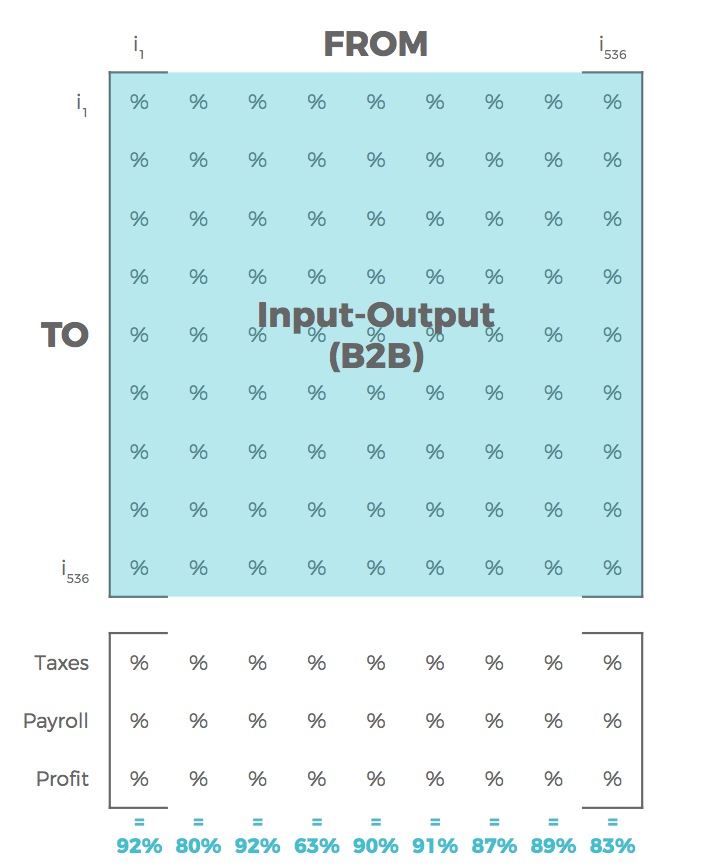
Each industry purchases Commodities from Industries to operate their business, which generates the initial round of backward linkages for each industry. Each cell in the matrix below represents a payment from the Sector column to the Commodity row. In other words, the dollars spent by a given Industry to purchase operational Inputs is represented by the columns in the matrix below. These dollars are referred to as Intermediate Expenditures. IMPLAN’s data source on Input purchases by Industry is only available at the National level. IMPLAN is an annual model so the input-output data in the matrices will be based on a given year. Intermediate Expenditures for each Industry can be converted to a Spending Pattern by dividing each expenditure by the total value of all Intermediate Expenditures for the given Industry, producing a percentage for each Intermediate Expenditure or the Gross Aborsportion that sum to 100% for the given Industry.
HOW ARE SECTOR PRODUCTION FUNCTIONS ARE REGIONALIZED:
Industries of course spend money on things other than Intermediate Expenditures. The Production Function of a Sector in IMPLAN determines how a Sector will allocate Output to continue to operate. To complete each Sector’s Production Function, we’ll need to incorporate the other production values. Industries must pay taxes. They also require Labor to create the final good or service. The Production Function also leaves room for profit to be earned and to cover things like the purchase of equipment. These additional factors of a sector’s Production Function are called Value Added. The combination of a Sector’s spending on Value Added and Intermediate Expenditures equals the Sector’s Total Output. IMPLAN collects sub-national data on Valued Added and Total Output by Sector.
Using regional dollar values for Total Output and Value Added for each Sector, a Value Added Coefficient can be calculated (Value Added / Total Output). Knowing the Production Function represents 100% of the distribution of total Output for a Sector, this regional Value Added Coefficient is used to adjust the National Spending Patterns so that the sum of the coefficients allocated to each Commodity purchase, Total Gross Absorption, plus the Value Added Coefficient, equals 100%, while maintaining the ratio of the Commodity purchases to one another.
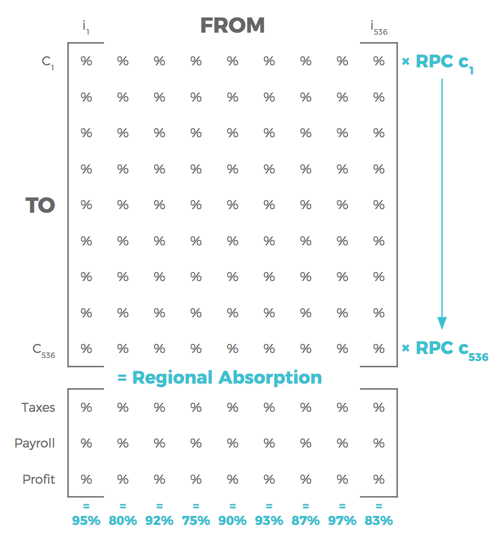
These regionalized Spending Patterns are further regionalized by converting Gross Absorption to Regional Absorption. The Commodities purchased by each Sector cannot all be sourced from within a closed economy; some Commodity purchases are imported from other regions. Therefore, each Commodity has a model-specific Regional Purchasing Coefficient.
Multiplying each Gross Absorption for a Sector by the Commodity’s RPC produces the Regional Absorption for the Sector and Region. The sum of Regional Absorption and the Value Added Coefficient for each Sector will be less than 100%. Because an RPC tells us how much demand is sourced locally, 1 minus the RPC tells us how much demand will be sourced non-locally, according to the model for each Commodity. You can think of this 1-RPC value as the import rate of the Commodity in the Region. The difference between 100% and the sum of Regional Absorption and Value Added for each Sector is the portion of dollars IMPLAN will model as leaving the Region when the effect of production in each Sector is analyzed. Dollars that model does not continue to circulate through the Region’s economy are considered leakages. The import of Commodities is one form of leakage.
CONVERTING COMMODITIES TO INDUSTRIES:
Recalling the definition of backward linkages, these linkages are from Industries to other Industries, but our matrices currently maps Industry’s purchases of Commodities, so IMPLAN converts Commodities to Sectors. This is another way in which regionality is factored. Commodities in IMPLAN are numbered 3001 through 3536 to distinguish them from Sectors. The Sector number for the primary producer of a Commodity can be translated by removing 3000 from the Commodity number, but Commodities can be sold/purchased from multiple sources. For some Commodities there are multiple producers and some Commodities can be stored in inventory and sold in a later year. Therefore, Commodity Output can be tied to production by a Sector or Sectors, and/or sales by an Institution (which includes inventory). The sum of the sources of a Commodity is called Commodity Supply. The portion of Commodity Supply that comes from each of these sources is called a Market Share. These Market Shares are based on the Commodity value from each source divided by the total value of the Commodity Supply. The Commodity value from each source and the Commodity Supply are specific to the Data Year and Region. Therefore, to convert the Regional Absorption for each Commodity to be Sector based, the Regional Absorption is distributed to the suppliers of the Commodity based on the Market Shares (found in Region Details > Social Accounts > Balance Sheets > Commodity Balance Sheet > Industry-Institutional Production). Through this conversion, the y-axis will become Sectors 1 through 536 and a new Sector based Spending Pattern is produced for each Sector. A Sector could be producing more than one Intermediate Expenditure Commodity, meaning they may make up some of the Market Share for more than one Commodity in a given Sector’s Spending Pattern. The portion of production dedicated to producing each commodity in a given Sector is called a Byproduct Coefficient (found in Region Details > Social Accounts > Balance Sheets > Industry Balance Sheet > Commodity Production).
Market Shares allocated to Institutions will not be modeled as continuing to circulate through the Region’s economy, treating these portions as a leakage.
The leakage due to institutional sales further decreases the sum of the Production Function for each Sector. This conversion makes the top matrix a true business to business Input-Output Matrix.
EXPANDING THE MODEL:
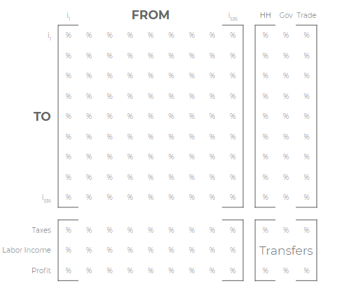
The Income earned by individuals working to produce a sector’s output also affects the economy when that Income Is spent. Incorporating these effects classifies the IMPLAN model as a Social Accounting Matrix (SAM) Model.
To incorporate Households and Institutions into the model, an additional matrix for Final Demand is added. Final Demanders are, by definition, Institutions. Final Demand is the value of goods and services produced and sold to final users to meet demand, whether it is local demand or an export. Final Demand for the Region can be found in the Region Details > Overview > Final Demand table.
Particularly in the case of government purchases, some of these purchases can be incorporated in creating some other good or service, such as materials purchased to build a new highway.
To determine how payroll transitions from compensation to disposable income, a final fourth matrix is added, completing the larger matrix. Considering the spending of Income allows for further regionalization of the model. The full cost of Labor is called Labor Income in IMPLAN.
Not all dollars earned by an individual or household are spent by the household. There are several ways in which some dollars earned leak out of the model. All Labor Income, regardless of which sector it was earned in, cycles through the model in the same way. The Employee Compensation and Proprietor Income columns, summing together to be Labor Income, make payments to the rows. Converting these column values from dollars to percentages of the column total gives us a pattern for the region and year that reflects the transfer of dollars earned as Labor Income to Household Income dollars.
Labor Income is distributed to the Household Income groups based on the percentage each of type Labor Income paid to each Household Income Group. Labor Income also makes payments to the Federal Government and may make payments to the State and Local Government depending on the Region. These are the payment of Payroll Taxes from Labor Income. Again, since we don’t know how, where, or when the government will use fiscal revenue, taxes paid are treated as a leakage and do not continue to circulate in the Region’s economy in the model.
The region specific in-commuting rate is also applied to Labor Income paid to wage and salary workers to leak income earned by non-residents out of the model. The in-commuting rate is the portion of Employee Compensation that will be estimated to leak out of the Region due to employees earning income within the Region, but commuting home, outside of the Region, where they spend their money (Region Details > Social Accounts > I x C Social Accounting Matrix > I x C Aggregate SAM > EC column, Foreign and Domestic trade rows divided by column total). These columns will always be blank for Proprietor Income as it is assumed to be earned by residents of the Region.
Income earned by Households locally is distributed to IMPLAN’s nine Household Income groups (categorizing ranges of income).
The journey of Household Income, the payment to Household rows from Labor Income, continues in the Household columns. Household Income primarily makes a payment to Commodities. Households also transfer money to other households. Personal taxes are reflected as the payment to government rows from the Household Income Group columns. Savings of household income is reflected as the payment to the Capital row from the Household Income Group columns. Converting these column values of payments to government and capital to percentages of the column totals gives us the effective Personal Tax and Savings rates, respectively.
We can break down the purchase of Commodities for each Household Income Group in Region Details > Study Area Data > Household Commodity Demand. Converting each Household Income group column from dollars to percentages of the column totals give us the Spending Pattern for each Household Income group. Like Sectors’ purchases of Commodities, the amount of each Commodity purchased by households that will be modeled as a local purchase is also determined by the Commodity’s RPC. Applying the average RPC for each Commodity would reflect the local spending per dollar of Household Spending on each Commodity. This information is reflected in dollars in Region Details > Social Accounts > Reports > Household Local Commodity Demand. The Commodities purchased by Households are converted to purchases to Sectors also using the Market Shares.
https://implan.com/wp-content/uploads/Market-site-Logo-resized-2-1.jpg00Adam Smithhttps://implan.com/wp-content/uploads/Market-site-Logo-resized-2-1.jpgAdam Smith2019-10-24 16:17:452019-10-24 16:17:57Sector Production Functions in IMPLAN