Local Industries Buying Local

INTRODUCTION

Did you ever wonder how much local bread your local supermarkets buy? Or how much local auto manufacturers spend on local tires? The process to find this answer may seem complicated, but it is actually relatively simple. Here’s how.


THE PROCESS

Let’s examine how much local beer is purchased by local restaurants in Greater Milwaukee. Start by selecting your Region (Milwaukee-Waukesha, WI MSA 2018 shown below) and heading into the data for Commodity 3106 – Beer, ale, malt liquor and nonalcoholic beer.


STEP 1: FIND THE TOTAL COMMODITY SUPPLY

Behind the i

     > Social Accounts

          > Reports

               > Commodity Summary

                    > Total Commodity Supply

Local_Buying_Local_-_Total_Commodity_Supply.jpg


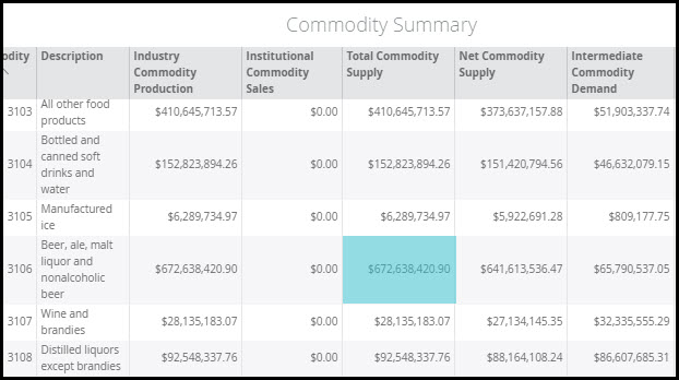
The Total Commodity Supply for beer is $672,638,420.90. This represents the total beer supply produced in Milwaukee by both Industries and Institutions.


STEP 2: FIND THE REGIONAL INPUTS

Behind the i

     > Social Accounts

          > Balance Sheets

               > Industry Balance Sheet

                    > Commodity Demand

                         > Filter for Industry 509 – Full-service restaurants

                              > Regional Inputs

Local_Buying_Local_-_Regional_Inputs.jpg

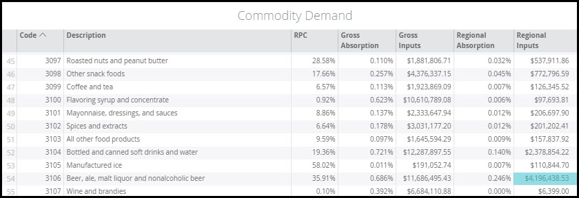
Scroll to Commodity 3106 – Beer, ale, malt liquor and nonalcoholic beer and find the value for Regional Inputs. For the Milwaukee-Waukesha, WI MSA this is $4,196,438.53. Regional Inputs show the amount that restaurants spend locally on beer during the Data Year. Note that the Gross Inputs of $11,686,495.43 represent the total annual spending on beer by full-service restaurants. We then know that local restaurants are spending 35.91% of their beer budget on local brews (RPC = 35.91%).


STEP 3: DIVIDE THE RESULTS

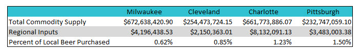
The Regional Inputs of $4M divided by the Total Commodity Supply of $673M tell us that Milwaukee restaurants are buying less than 1% of total local beer production. Given how much beer production occurs in the Region, the percentage of local beer production that is purchased by local restaurants is quite low. The table below compares four cities on the percentage that local restaurants spend on local beer.

Local_Buying_Local_-_4_City_Comparison.jpg

STEP 4: EXAMINE EXPORTS

Behind the i

     > Social Accounts

          > Reports

               > Commodity Trade


Local_Buying_Local_-_Commidty_Trade.jpg

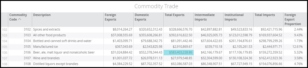
Now we can look at exports. Foreign Exports tells us the total local production that is exported outside the U.S. The Domestic Exports tells us the total local production that leaves Greater Milwaukee but stays in the U.S. The Total Exports is a combination of these two. The Total Exports from Milwaukee is $583,403,228.86. Taking this divided by the Total Commodity Supply of $672,638,420.90 tells us that 87% of the locally produced beer is exported from the MSA. Therefore, 13% stays local – which is known as the Average RSC (Regional Supply Coefficient). 


STEP 5: INCREASE LOCAL BEER PURCHASES

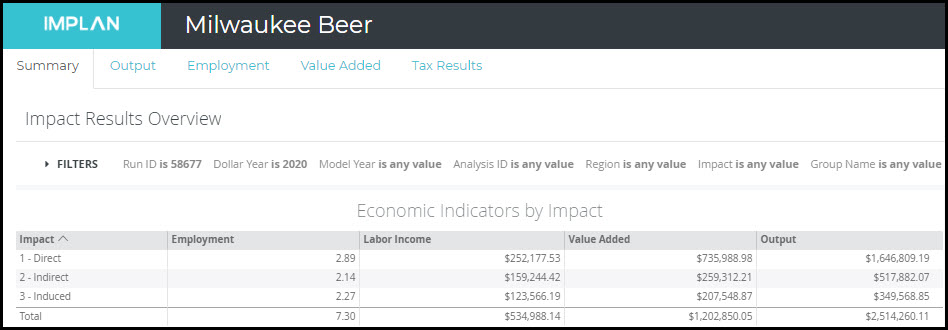
Let’s say local restaurants want to commit to purchasing a full 50% of their beer from local breweries. They are currently spending a total of $11,686,495.43 on beer, so half would be $5,843,247.72. They are currently spending $4,196,438.53, so they would need to increase their local buy by $1,646,809.19. We can run this as an Industry Output Event.


Local_Buying_Local_-_Impacts.jpg

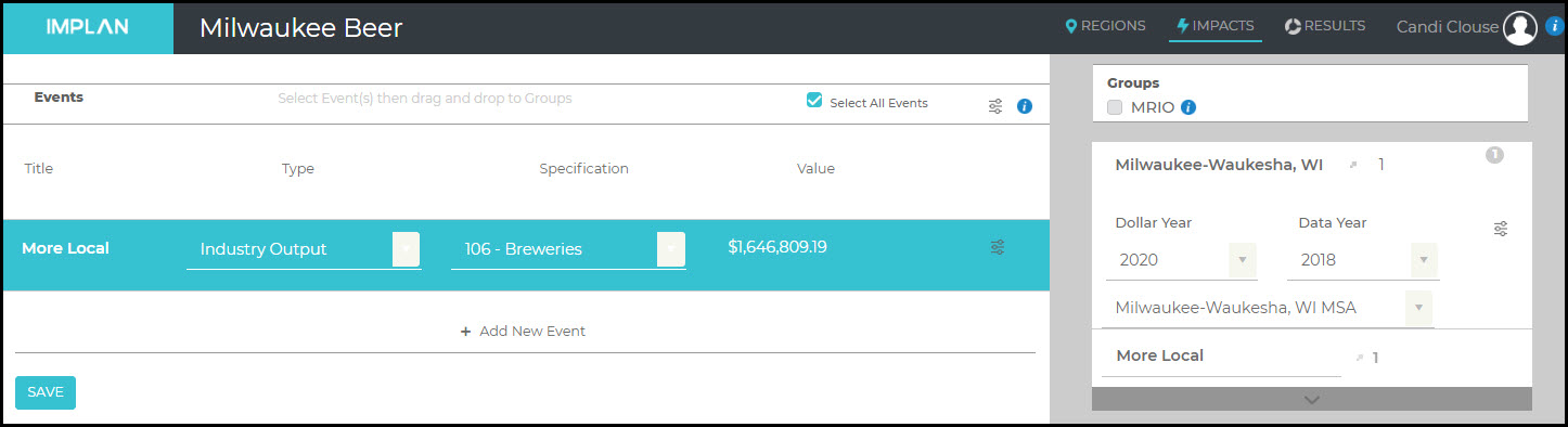
The Results show us that the increase in $1,646,809.19 in local breweries supports a total Output of $2,514,260.11; a multiplier of 1.53. This will support almost 3 employees at the brewery and 4 additional employees in the Indirect and Induced Effects; a multiplier of 2.53.

Local_Buying_Local_-_Results.jpg


RELATED ARTICLES

Behind the i

Deflators

What are deflators and when are they used in IMPLAN?

The purchasing power of a dollar changes over time (typically decreasing) due to inflation, a cyclical phenomenon by which prices of goods and services increase[1], which spurs workers to demand higher wages, which in turn increases demand for goods and services, thereby spurring additional price increases, and so on.  Due to inflation, a dollar in 2017 cannot purchase as much as did a dollar in 2001, for example; as such, a 2017 dollar is not the same thing as a 2001 dollar.  IMPLAN’s deflators are indexes of inflation, with the deflator for the model data year set at 1.00. 

The deflators are not used to create the social accounts or multipliers but are necessary for impact analysis whenever the dollar year of the event differs from the year of the model data.  The same model year multipliers are used regardless of the dollar year of the event; it is the value applied to those multipliers that changes when the dollar year of the event differs from the year of the model data.  Indeed, if one were to run an un-customized event using an event year that differs from the model year but views the results in the same year as the model, the multipliers calculated from these results will match the multipliers displayed in the multipliers tables of the model.

Why is this adjustment needed?

All the relationships in the multipliers are based on model year prices, so the direct effects applied to those multipliers need to also be in model year dollars – this is accomplished via the deflators.  The value applied to the multipliers is the user-entered value divided by the deflator.  The deflators also allow impact results to be viewed in years other than the model year, regardless of whether or not the dollar year of the event differs from the year of the model data. 

While the event values and/or result values can be inflated or deflated, depending on whether the index value being applied is less than 1.00 or greater than 1.00 (i.e., depending on the industry/commodity and whether one is adjusting to a future or past value), we use a single term – deflators – to refer to all of these index values.

The output deflators are specific to the industry/commodity and are applied to the output value, while the same GDP deflators are the same for every industry/commodity and are applied to all of the value-added components.

Source data

The Bureau of Economic Analysis (BEA) provides historical output deflators which we use for past to current years.  For projections into the future, we use the annual rate of change from the Bureau of Labor Statistics’ (BLS) employment growth model.  The BEA also has historical GDP deflators which we use for past to current years.  For projections into the future, we use the annual rate of change from the BLS employment growth model for “All Industries”. 


[1] Not all goods and services are inflationary every year.  For example, the prices of consumer electronics often decrease over time.  As another example, the prices of agricultural commodities rise and fall in response to many factors, including weather.