Multipliers Changing Over Time

INTRODUCTION

IMPLAN introduces new data each year. With new data, comes new multipliers. In general, it is not advisable to treat annual IMPLAN datasets as a time series as our data sources and methods often change from year to year.  Additionally, some of our raw data sources revise estimates, so that, for example, what a source reports about 2013 in 2018 is different from that source would report about 2013 in 2019. This is especially true of data from the Bureau of Economic Analysis. On a 5-year basis (following the incorporation of a new BEA Benchmark, Census of Agriculture, and IMPLAN Industry scheme) we publish Panel Data, spanning from 2001 to the latest annual IMPLAN data year, to facilitate year-over-year analysis.  These datasets use all the data and methodological changes incorporated over the preceding 5 years, and are reported in the same (latest) IMPLAN sectoring scheme. 


DETERMINING MULTIPLIER SIZE

Again, as the data changes over time, it is not uncommon to see changes in the multipliers. Changes of less than 10% (positive or negative) are quite routine and expected. Larger changes can be expected if comparing non-consecutive years or years that span one of our 5-year data sets (see next section on Five Year Data).  Employment and Value Added multipliers can vary greatly across geographies and years whereas Output multipliers tend to be relatively more stable.

Multipliers are influenced by many factors, so it is not possible to isolate a single factor when examining their changes over time. These factors include some that are specific to the geography in question, while others are specific to the Industry in question. Still others may be related to global trends. Here are some reasons why there are yearly changes.

  • A greater reliance on imports (whether foreign or domestic) will result in lower RPCs in general, which, all else equal, reduce multipliers. 
  • When productivity, as defined as Output per worker, rises in a given Industry, the Employment per dollar of Output falls. All else equal, a smaller Direct Employment will result in a larger Employment multiplier for this Industry.  
  • Change in Labor Income per dollar of Output, whether from changes in wage rates or the changing fortunes of proprietors, will change the magnitude of Induced Effects, and therefore multipliers. Proprietor Income can be negative and can vary substantially from one year to the next. 
  • A decrease in a multiplier can also be caused by a large increase in corporate profits and/or taxes paid per dollar of Output. Corporate profits make up the bulk of Other Property Income (OPI), a component of Output that is treated as a leakage in I-O modeling, in the sense that they are not spent within the model and therefore do not generate Indirect or Induced Effects.  Similarly, all taxes, while accounted for in the tax impacts report, do not generate additional rounds of impacts. The larger the percentage of Output that goes to OPI and taxes, the less leftover to drive Indirect and Induced Effects.


FIVE YEAR DATA

Some raw data sets are released only every 5 years; thus, larger year-over-year changes can be expected when comparing IMPLAN data across two years that span the release of one of these 5-year data sets, like between 2017 (536 Industry Scheme) and 2018 (546 Industry Scheme).

THE BEA BENCHMARK I-O TABLES – RELEASED EVERY 5 YEARS

A new BEA Benchmark provides new industry spending patterns for all IMPLAN industries.  The magnitude of total Intermediate Input purchases per dollar of Output and the relative mix of input purchases both influence Indirect Impacts, and the Induced Impacts associated with those Indirect Impacts.   

A new BEA Benchmark also provides data on the foreign imports and exports of Commodities. While we have annual Census data for the foreign trade of all shippable Commodities, no such data source exists at this level of Commodity detail for the annual foreign trade of services.  Thus, we turn to the BEA Benchmark to give commodity detail to the NIPA control total for the foreign trade of services.

A new BEA benchmark also provides new national indicators of the relationship between Output, Employee Compensation, gross operating surplus (PI + OPI), and TOPI.  These relationships are especially important for farm data, as many of our annual sources report data for agriculture only at the farm level. We use the BEA Benchmark for other components, including detailed Commodity margins, which will have more minor effects on multipliers. 

THE CENSUS OF AGRICULTURE – RELEASED EVERY 5 YEARS

The Census of Agriculture provides us with data on farm counts (both proprietor-owned and corporate-owned) by farm sector, by county. These data are used annually to distribute state-level farm Output data to counties and to provide Industry detail to the aggregate farm BEA REA data we use for farm Industry Employment and Labor Income. 


INVESTIGATING A CHANGE

If you see a change in multipliers that has you curious, here are four steps to investigate what may be causing it.

STEP 1: PRELIMINARY CHECKS 

  • Are both data sets in the same Industry Scheme? 
  • Is any aggregating or splitting needed to make the Industries comparable?

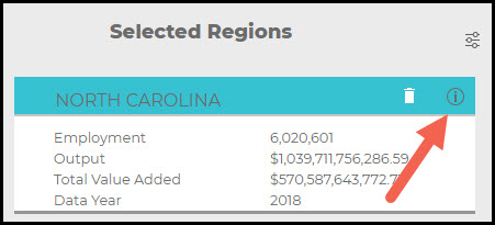
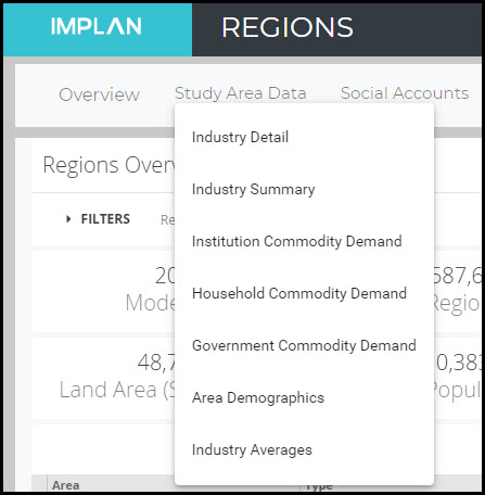
STEP 2: EXAMINE THE STUDY AREA DATA

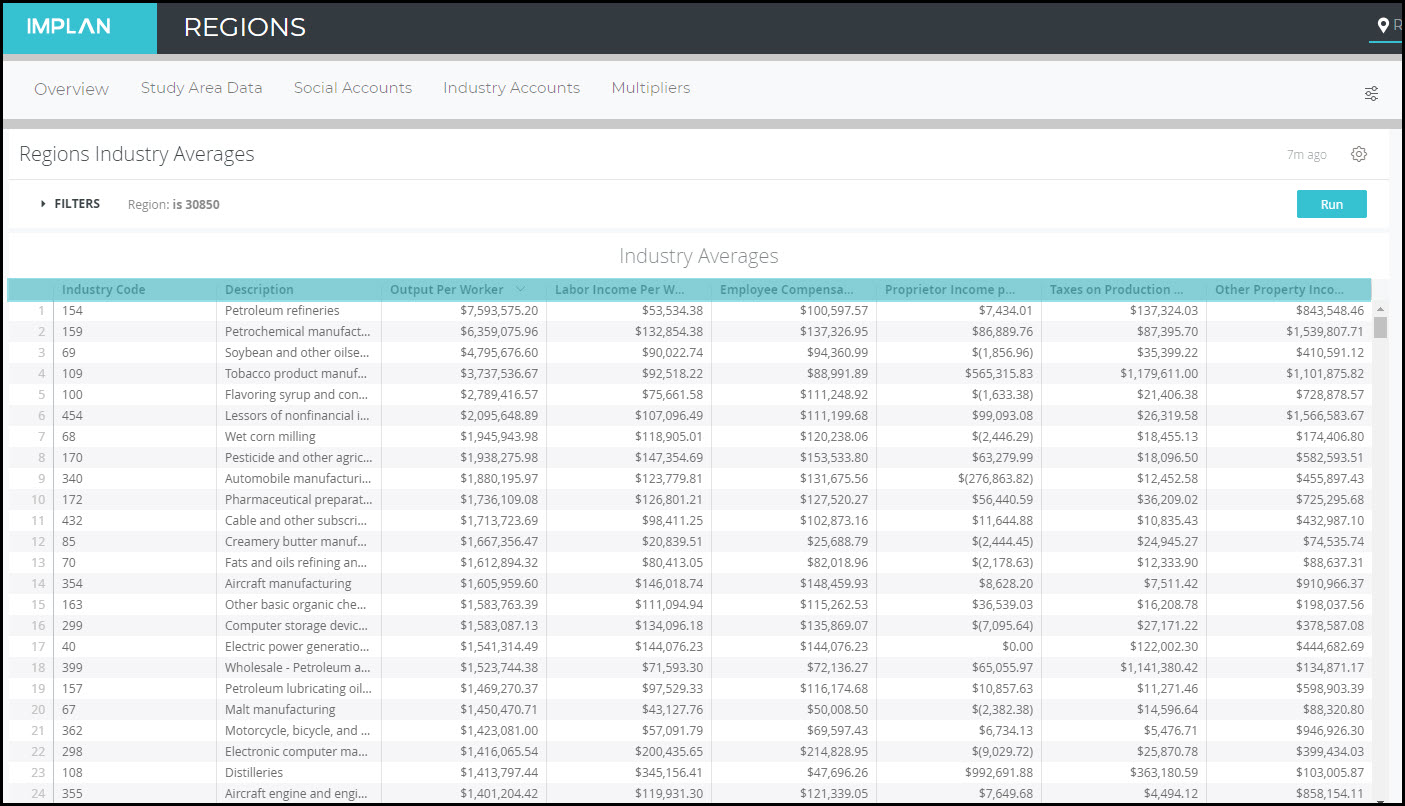
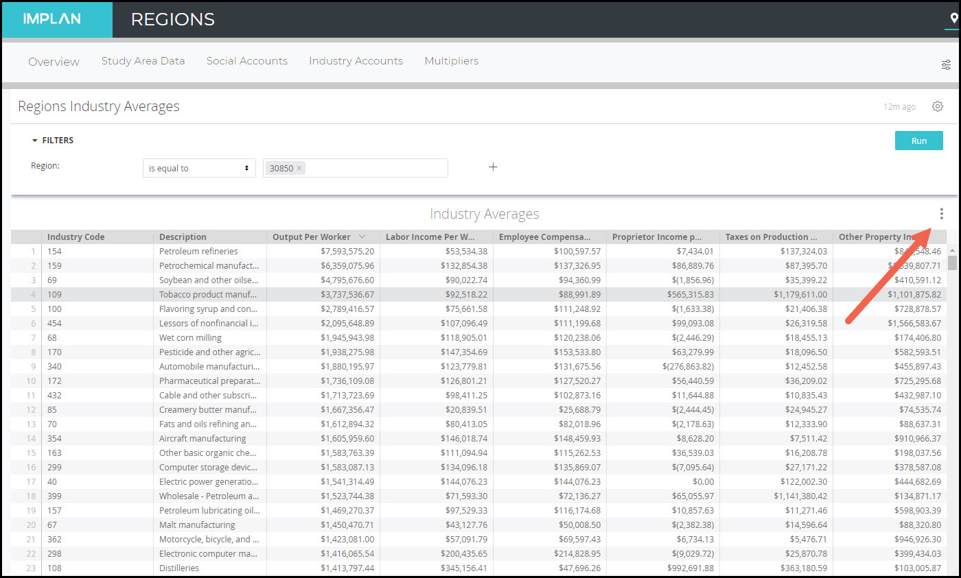
  • Has Employment per Output changed significantly?  
  • Has Labor Income per Output changed significantly?

STEP 3: EXAMINE SPENDING PATTERN AND RPCS OF TOP ITEMS

  • Has the ratio of Intermediate Inputs per Output changed significantly?
  • Have the RPCs of the top few Commodities purchased by the Industry changed significantly?

STEP 4: CONTACT IMPLAN SUPPORT FOR ASSISTANCE

Help us help you!  To expedite the process of investigating a value, it is extremely helpful for us to have the following details at the outset:

  • What type of multiplier are you concerned with (Employment, Output, etc.)?
  • What specific IMPLAN Industry or Industries, with the associated Industry number(s) are in question?
  • What are the two data years being compared?
  • What is the geography in question?
  • Is the multiplier in question from the Multipliers Report in IMPLAN or calculated based on impact results?

Then shoot an email to support@implan.com and our Data Team will take a look!


RELATED ARTICLES

BEA Benchmark & The New 546 Industry Scheme

IMPLAN Annual Data Updates

Multipliers

Negative Multipliers

Panel Data

Understanding Multipliers

Region Details: Behind the “i”

ABP: Analysis-by-Parts & Bill of Goods Using Commodity or Industry Events with Labor Income Event(s)

INTRODUCTION:

Analysis-by-Parts (ABP) is a technique by which you can split the “stemming ripple effects” of an event into its individual impact components – in this case if you have spending by line item and income. Separating the pieces with Analysis-by-Parts gives the researcher more flexibility and customization capabilities in the analysis. 

DETAILED INFORMATION:

To perform an Analysis-by-Parts using a bill of goods approach, you will want to know Direct Labor Income and the budget details.  Many times, you may be given the budget by the client that outlines their total spending along different businesses or products. This information can be directly translated into Events in IMPLAN.  

STEP 1 – EXPENDITURES

In the bill of goods approach, the researcher is presented with a budget.  This will either contain a list of companies from which the institution or industry purchases things (industries) or a list of the items that it purchases (commodities).  The researcher will need to first determine if they will be modeling Commodities or Industries.

  • A Commodity is a product or service that may be produced by one or by many industries.
  • An Industry represents a group of establishments engaged in the same or similar types of economic activity.

Next, choose the Specification that best matches each line item of purchase either by IMPLAN Sector code or IMPLAN Commodity code.

Enter each line of spending as either a Commodity Output Event or an Industry Output Event.  There will be many different Event lines in the model.

  • Remember to apply Margins  as necessary
    • When you have expenditure data by Industry, retail/wholesale purchases can only be modeled via the retail or wholesale Sectors. Only retail/wholesale industries can be margined.  If the expenditure value is a full retail sales value, you can leave the Margin default setting of “Total Revenue,” which will apply margins to the expenditure value. The estimated retail margin will then get applied to the retail Multipliers. The wholesale and transportation margins, as well as the production value will be leaked out of the model.
    • When you have expenditure data by Commodity and the expenditure value is the retail sales value of the Commodity, margins should be applied. Again, in this case you can leave the Margin default setting of “Total Revenue,” which will apply margins to the expenditure value. For Commodities, marginning will estimate not only the retail margin, but also the wholesale and transportation margins, along with the production value. Here, nothing will be leaked out of the model except for any Commodity Supply that will come from Institutional Sales or Inventory.
    • Changing the Margin selection to “Marginal Revenue” indicates you are entering the producer price, the producer being indicated by the Specification on the Event. For Commodities and Industries that are not marginable “Marginal Revenue” will be the only option.

If you need to make adjustments to IMPLAN’s margins, learn more about Manually Margining.

  • Also remember to appropriately specify the portion of the purchase that is coming from local production
    • Adjust Local Purchase Percentage (LPP) for Commodity Output Events as necessary. If we know the Commodity will be produced in the Region we will leave the Local Purchase Percentage at 100%. If we don’t know where the purchase was produced (which is often the case), setting Local Purchase Percentage to SAM is most appropriate. You can also enter your own known percentage for the portion of the purchase that will be local. 
    • For purchases by Industry, only purchases from local businesses should be modeled and included in the Industry Output Event Values.  

For example, let’s say a small dog treat bakery is opening up in North Carolina.  We know what items they will purchase (commodities) to operate their store.  

  1. Since the purchased Commodities are known, each purchased Commodity will be entered as a Commodity Output Event.
  2. For each of these items, we will find the appropriate Commodity code.  Peanut butter is commodity code 3099 – Roasted nuts and peanut butter manufacturing, as an example.  Repeat this step for each of the Commodities that will be purchased.  
  3. All of the bakery’s retail purchases should have margins applied by leaving the selection of “Total Revenue.” Since the place of production would likely be unknown, LPP should be set to SAM. Other purchases, such as local utility payments would have the selection of “Marginal Revenue” because the amount the bakery pays for these Commodities is a Producer Price. For payments to utility providers in the Region, LPP should be left at 100%.

A more simple alternative approach, as opposed to modeling each Intermediate Expenditure, is to run the total Intermediate Expenditures value through the Industry Spending Pattern that best reflects the industry you are modeling. For this approach, follow the instructions for Analysis-by-Parts: Using an Industry Spending Pattern Event with Labor Income Event(s).

STEP 2 – LABOR INCOME

Next, a Labor Income Event must be created either for Employee Compensation (EC), Proprietor Income (PI), or both.

In our example, the bakery will be run by the owner (proprietor) who will receive $75,000 in labor income and one additional employee that will receive $55,000.  A Labor Income Event will be created for each: $75,000 for Proprietor Income and $55,000 for Employee Compensation.  

Remember, these should be fully loaded payroll values which include wage and salary, all benefits (e.g., health, retirement) and payroll taxes (both sides of social security, unemployment taxes, etc.).  

If you need to convert your wage and salary data to fully loaded payroll, please use the 536 FTE & EMPLOYEE COMPENSATION CONVERSION TABLE.

BOE1.png

STEP 3 – RUN THE IMPACT

Now either use the button at the top to select all or highlight each Event and drag them into your Group.  Next, hit run.

BOE2.png

STEP 4 – INTERPRET THE RESULTS

When your analysis is complete, the results will show you the economic impact of all of the Events you entered which will include the Commodity or Industry Events  and the Labor Income Event(s).

In our Dog Bakery example, this investment has an economic impact of almost 21 jobs, $840,500 in Labor Income, $1.4 million in Value Added, and $3.1 million in Output.

  • The Direct and Indirect Effects are from the Commodity/Industry Events only and represent employment in the local industries directly affected (via a purchase from within the Direct business’s supply chain, in this example, the dog treat bakery).
  • The Labor Income events only create Induced Effects.

If you want to look at the results by Event, remember to use the FILTERS button and select which of the Events you would like displayed.

BOE3.png

STEP 5 –  MODIFYING RESULTS

Because your Direct Effects are from the Commodity/Industry Events, which only reflect the purchases made by the true Direct business, the Results should be modified. Your Direct Effects are actually Indirect Effects. 

  • Subtract you Direct Effect from your Direct Effect so the Direct Effects become all zeros. 
  • Add these Direct Effects to the existing Indirect Effects to generate a new Indirect Effect.
  • Define your Direct Effect:
    • Direct Labor Income = total Labor Income. You should use the values run through the Labor Income Event(s) from Step 2.
    • Direct Value Added = Direct Labor Income + Tax on Production and Imports + Other Property Income
      • This can also be derived from the Output equation in the model:
        • If you have Output, you can use the equation Value Added = Output – Intermediate Expenditures (the sum of your expenditures)
        • If you only have sum of expenditures and Direct Labor Income, you’ll need to find out how these values relate to Value Added in the Output equation for the Sector that best represents the Direct Industry, in Region Details > Social Accounts > Balance Sheets > Industry Balance Sheets
          • Using the Value Added Tab, Value Added can be calculated as (Labor Income/Labor Income Coefficient) * Value Added Coefficient.  The Labor Income Coefficient being a sum of EC and PI Coefficients. 
          • Value Added could also be calculated using the Commodity Demand tab, Gross Absorption column total and Value Added Coefficient as (sum of expenditures)/Gross Absorption Coefficient * Value Added Coefficient 
          • Note that if these two approaches produce different results it is because your sum of expenditures and Labor Income values don’t follow the same ratio to one another as the Output Equation suggests and some assumptions about how your Output Equation differs will need to be addressed. 
    • Direct Output = Sum of all expenditures (Intermediate Expenditures) + Direct Value Added
    • Direct Employment = known Direct Employment, in this example, we already know there are only 2 Employees. If Employment is unknown, you can calculate it on your own by dividing Direct Output by Output-per-worker for the Sector that best represents the Direct Industry. Output-per-worker can be found by Sector in Region Details > Study Area Data > Industry Summary. 


RELATED TOPICS:

ABP: Introduction to Analysis-By-Parts

ABP: Analysis-by-Parts Using an Industry Spending Pattern Event with Labor Income Event(s)

ABP: Analysis-by-Parts with Manually Margining Bill of Goods

Hospitals: Modeling Private Hospital Impacts with Analysis-by-Parts

Hospitals: Modeling Public & Nonprofit Hospital Impacts with Analysis-by-Parts

Proving Analysis-By-Parts: A Comparison of Event Types

Multipliers

INTRODUCTION:

Multipliers are the total production impact within the Study Area for every unit of direct production. Total production will vary depending on the method of inclusion (whether the Induced Effects are included or not). There are four (4) Multiplier View By Options: OutputEmploymentLabor Income, and Value Added.  Value Added can be further split into Employee Compensation, Proprietor Income, Other Property Income, and Tax on Production and Imports.

The calculations or method of inclusion used to create Type I and Type SAM Multipliers are shown below:

     Type I Multiplier = (Direct Effect + Indirect Effect) / (Direct Effect)

     Type SAM Multiplier = (Direct Effect + Indirect Effect + Induced Effect) / (Direct Effect)


SUMMARY MULTIPLIERS:

Multipliers_-_Summary.jpg

Output shows the Multipliers used to generate Output effects
Employment provides Employment Multipliers per million dollars of Output
Labor Income displays Labor Income Multipliers per million dollars of Labor Income
Value Added shows the summed Multipliers for all Value Added types per million dollars of Value Added
Employee Compensation shows the Multipliers used to create Employee Compensation portion of Labor Income impacts
Proprietor Income displays Proprietor Income Multipliers for calculating the Proprietor Income portion of Labor Income
Other Property Income provides Multipliers for calculating OPI taxes
Tax On Production and Imports provides Multipliers for calculating TOPI taxes


DETAIL MULTIPLIERS:

The Detail Multiplier view breaks down each Multiplier by: Type I, Induced, and Type SAM for each view by: OutputEmploymentLabor Income, and Value Added as they are applied to Industry x Industry Input/Output transactions. Select an Industry Sector from the drop down menu to see updated total values for Type I, Induced, and Type SAM Multipliers for the selected industry. 

     Type I Multiplier = (Direct Effect + Indirect Effect) / (Direct Effect)

     Type SAM Multiplier = (Direct Effect + Indirect Effect + Induced Effect) / (Direct Effect)

     Induced Multiplier = Type SAM Multiplier – Type I Multiplier

Multipliers_-_Detail.jpg

In the Regions Multipliers Detail, the default Industry or Commodity is always Oilseeds.  In order to see the Industry or Commodity of interest, click the Filter button and choose the appropriate Sector.  Click Run to have the model filter for that Sector.

Social_Accounts_-_Filter.jpg

Output shows the Multipliers used to generate Output effects
Employment provides Employment Multipliers per million dollars of Output
Labor Income displays Labor Income Multipliers per million dollars of Labor Income
Value Added shows the summed Multipliers for all Value Added types per million dollars of Value Added
Employee Compensation shows the Multipliers used to create Employee Compensation portion of Labor Income impacts
Proprietor Income displays Proprietor Income Multipliers for calculating the Proprietor Income portion of Labor Income
Other Property Income provides Multipliers for calculating OPI taxes
Tax On Production and Imports provides Multipliers for calculating TOPI taxes


SORTING:

The title bar displayed across the top of each Study Area View By contains buttons that can change the viewing attributes of the table. The bar shown is for Output Multipliers.

Multipliers_-_Sort.jpg

Most column titles act as sorting buttons. Initially most views are sorted by Sector code in ascending value (first row is 0 last row is 546). To change the way all fields in the table are arranged, click on the title of the desired column. All data in the table will be sorted in descending order (highest values listed at the top of the table) relative to the column title. To change how the data is sorted, click on another field. When the view has been sorted by a column other than Industry Code, the selected column title will appear with an arrow to its right indicating that the table has been sorted by this column header.


DOWNLOADING:

The export function allows data to be exported directly to a PDF or CSV file by clicking on the gear icon.

Industry Accounts

REPORTS:

Industry_Accts_-_Reports.jpg

Institution Industry Demand shows the distribution of each Industry’s production to Institutions, Capital, Inventory, and Exports from Study Area Industries.

Household Industry Demand divides the total Household’s consumption, provided in Institution Industry Demand, into the 9 Household income classes.

Government Industry Demand expands the government consumption into the three Federal and three State and Local government types.

Industry Output/Outlay Summary shows total Industry expenditures and receipts. Purchases are detailed by Industry (Intermediate Outlay), Institution, Imports, and Value Added, while receipts are broken into Intermediate Output and Final Demand.


IxI SOCIAL ACCOUNTING MATRIX:

Industry_Accts_-_IxI.jpg


Aggregate IxI SAM (rows and columns are aggregated) provides an overview of the entire IxI Social Accounting Matrix. Categories in both rows and columns show totals for all types of monetary transactions.

Detail IxI SAM columns remain aggregated; however, rows are presented with Industry, Value Added, Institutions, and trade transactions divided additionally by transaction types. 


SORTING:

The title bar displayed across the top of each Study Area View By contains buttons that can change the viewing attributes of the table. The bar shown is for Institution Industry Demand.

Industry_Accts_-_Sort.jpg

Most column titles act as sorting buttons. Initially most views are sorted by Sector code in ascending value (first row is 0 last row is 546). To change the way all fields in the table are arranged, click on the title of the desired column. All data in the table will be sorted in descending order (highest values listed at the top of the table) relative to the column title. To change how the data is sorted, click on another field. When the view has been sorted by a column other than Industry Code, the selected column title will appear with an arrow to its right indicating that the table has been sorted by this column header.


DOWNLOADING:

The export function allows data to be exported directly to a PDF or CSV file by clicking on the gear icon.

Social Accounts

INTRODUCTION:

The Social Account Reports Table and the Balance Sheets Table both contain a wealth of information about the specified study region. Provided below are definitions and descriptions of many of the terms and categories found within the tables.


REPORTS:

Social_Accounts_-_Comm_Summary.jpg

Commodity Summary

  • Industry Commodity Production = the total output of this commodity that is produced by industries. Some commodities are produced by more than one industry – this value includes the sum of the production of this commodity by all industries.
  • Institutional Commodity Production = the total output of this commodity that is produced by institutions (i.e., produced by Government or taken out of Inventory).
  • Total Commodity Supply = Industry Commodity Production + Institutional Commodity Production.
  • Net Commodity Supply = Total Commodity Supply – Foreign Exports of the commodity from the region. Foreign Exports can be found by selecting View By: Commodity Trade.
  • Intermediate Commodity Demand = total demand for this commodity by industries.
  • Institutional Commodity Demand = total demand for this commodity by institutions (Inventory, Government, Households, Capital).
  • Total Gross Commodity Demand = Intermediate Commodity Demand + Institutional Commodity Demand. The term “gross” refers to the fact that these figures include imports (both foreign and domestic) of the commodity into the region.
  • Domestic Supply/Demand Ratio = the percentage of total local demand for the commodity that could possibly be met by local production. It is calculated by dividing Net Commodity Supply by Total Gross Commodity Demand, constrained to a maximum of 100%.
  • Average RPC = the proportion of local demand for the commodity that is currently met by local production. It is “average” in the sense that there is just one RPC per commodity, so all industries and institutions are assumed to purchase that commodity locally at the same rate.
  • Average RSC = the proportion of local supply of the commodity that goes to meet local demand.

Commodity Trade

  • Foreign Exports = output value of local production of this commodity that is exported abroad.
  • Domestic Exports = output value of local production of this commodity that is exported to other regions of the U.S.
  • Total Exports = Foreign Exports + Domestic Exports
  • Intermediate Imports = value of imports (both foreign and domestic) into the region for use by industries as an input.
  • Institutional Imports = value of imports (both foreign and domestic) into the region for final use by institutions (Inventory, Government, Households, Capital).
  • Total Imports = Intermediate Imports + Institutional Imports.
  • Foreign Export Proportion = the percentage of Total Exports that go to foreign countries. It is calculated by dividing Foreign Exports by Total Exports.

Institution Local Commodity Demand

This table lists each institution’s demand for local production of each commodity. The sum across all institutions for a particular commodity is the total local institutional demand for local production of that commodity. Foreign Exports and Domestic Exports are the same as reported in the Commodity Trade screen.

Household Local Commodity Demand

This table lists each Household type’s demand for local production of each commodity. The sum across all Household types for a particular commodity is equivalent to the “Households” value on the Institution Local Commodity Demand screen.

Government Local Commodity Demand

This table lists each Government type’s demand for local production of each commodity. The sum across all six Government types for a particular commodity is equivalent to the “Government” value on the Institution Local Commodity Demand screen.


BALANCE SHEETS:

Social_Accounts_-_Comm_Prod.jpg

Industry Balance Sheet

On all of the Balance Sheets, the default Industry or Commodity is always Oilseeds.  In order to see the Industry or Commodity of interest, click the Filter button and choose the appropriate Sector.  Click Run to have the model filter for that Sector.

Social_Accounts_-_Filter.jpg

Commodity Production

  • Commodity Production = the output value of each of the commodities produced by this industry.
  • Market Share = the proportion of Commodity Production that is produced by this industry. If there is more than one producer of a commodity, this industry’s Market Share for that commodity will be less than 100%.
  • Byproduct Coefficient = the proportion of this industry’s total industry output that is dedicated to each commodity. If the industry makes more than one commodity, each Byproduct Coefficient will be less than 100%.

Commodity Demand

  • RPC = the proportion of local demand for the commodity that is currently met by local production. This is the same value as that found in the View By: Commodity Summary screen.
  • Gross Absorption = the proportion of Total Industry Output for this industry that goes toward purchases of each commodity. Gross Absorption is calculated as Gross Inputs/Total Industry Output. Total Gross Absorptions will be less than one, with the remainder of Total Industry Output going toward Value-Added.
  • Gross Inputs = the value that this industry spends on each commodity.
  • Regional Absorption = the proportion of Total Industry Output for this industry that goes toward local purchases of each commodity. Regional Absorption can be calculated as Gross Absorption * RPC.
  • Regional Inputs = the value that this industry spends locally on each commodity. Regional Inputs can be calculated as Gross Inputs * RPC.

Value Added

  • Value Added Coefficient = the proportion of Total Industry Output that goes toward each category of Value-Added. Each Value Added Coefficient can be calculated by dividing Value Added by Total Industry Output. The Total Value-Added Coefficient + Total Gross Absorption = 1.00.
  • Value Added = the dollar value paid to each category of Value Added.

Commodity Balance Sheet

Industry-Institutional Production

  • Industry Production = the total output of this commodity that is produced by the industry listed in each row.
  • Regional Market Share = the proportion of Industry Production that is produced by the industry/institution listed in each row. If there is more than one producer of this commodity, each Market Share will be less than 100%.
  • (Byproduct) Coefficient = the proportion of each industry’s total industry output that is dedicated to this commodity. If the industry/institution makes more than one commodity, the Byproduct Coefficient will be less than 100%.

Industry Demand

  • RPC = the proportion of local demand for the commodity that is currently met by local production. This is the same value as that found in the View By: Commodity Summary screen.
  • Gross Absorption = the proportion of Total Industry Output for each industry that goes toward purchases of this commodity. Gross Absorption is calculated as Gross Inputs/Total Industry Output.
  • Gross Inputs = the value that each industry spends on this commodity.
  • Regional Absorption = the proportion of Total Industry Output for each industry that goes toward local purchases of this commodity. Regional Absorption can be calculated as Gross Absorption * RPC.
  • Regional Inputs = the value that each industry spends locally on this commodity. Regional Inputs can be calculated as Gross Inputs * RPC.

Institutional Demand

  • RPC = the proportion of local demand for the commodity that is currently met by local production. This is the same value as that found in the View By: Commodity Summary screen. Note that if institutions purchase this commodity from local retailers, the retail margin portion of the purchase will have a high RPC; however, the producer portion of the purchase price will have a low RPC if there is little local production of that commodity.
  • Gross Demand = the amount that each institution spends on this commodity.
  • Regional Demand = the amount that each institution spends locally on this commodity. Note that this value has already been margined (that is, if the institution buys this commodity from a retailer, this value only shows the portion of that purchase amount that goes to local producers of the commodity). Regional Demand can be calculated as Gross Demand * RPC.


IxC SOCIAL ACCOUNTING MATRIX:

Social_Accounts_-_IxC.jpg

Aggregate IxC SAM& Detail IxC SAM:

Details on these tables can be found in the article: Summary Description of Elements of the IxC Social Accounting Matrix


SORTING:

The title bar displayed across the top of each Study Area View By contains buttons that can change the viewing attributes of the table. The bar shown is for Regions Commodity Summary.

Social_Accounts_-_Sort.jpg

Most column titles act as sorting buttons. Initially most views are sorted by Sector code in ascending value (first row is 0 last row is 546). To change the way all fields in the table are arranged, click on the title of the desired column. All data in the table will be sorted in descending order (highest values listed at the top of the table) relative to the column title. To change how the data is sorted, click on another field. When the view has been sorted by a column other than Commodity Code, the selected column title will appear with an arrow to its right indicating that the table has been sorted by this column header.


DOWNLOADING:

The export function allows data to be exported directly to a PDF or CSV file by clicking on the gear icon.

Social_Accounts_-_Download.jpg

Study Area Data

INTRODUCTION

Specific detailed information about your Region can be found in Study Area Data.  From the Regions screen, click on the letter i.

Study_Area_Data_-_Behind_the_i.jpg

The Study Area Data tab has seven options for exploring the data behind IMPLAN.


Study_Area_Data_-_7_Options.jpg


INDUSTRY DETAIL

This section shows Study Area Industry totals for the current values for the calendar year of the data in your Selected Region.

  • Total Output =  the value of Industry production, which is equal to sales plus net inventory change
  • Wage and Salary Employment = an Industry-specific mix of full-time, part-time, and seasonal employment excluding proprietors
  • Employee Compensation = the total payroll cost of the employee including wages and salaries, and all benefits
  • Proprietor Employment = an Industry-specific mix of full-time, part-time, and seasonal proprietor employment; excluding wage and salary employment
  • Proprietor Income = current-production income of sole proprietorships, partnerships, and tax-exempt cooperatives
  • Other Property Income = Gross Operating Surplus minus Proprietor Income
  • Taxes on Production and Imports = includes sales and excise taxes, customs duties, property taxes, motor vehicle licenses, severance taxes, other taxes, and special assessments

INDUSTRY SUMMARY

This table is a broader view of Industry contribution to the Selected Region, combining some Industry Detail values into higher classifications. 

  • Total Employment = an Industry-specific mix of full-time, part-time, and seasonal employment including both Wage and Salary Employment and Proprietor Employment
  • Total Output =  the value of Industry production, which is equal to sales plus net inventory change
  • Total Intermediate Inputs = purchases of non-durable goods and services that are used to produce other goods and services rather than for final consumption
  • Total Value Added = the difference between an Industry’s or establishment’s total Output and the cost of its Intermediate Inputs; it is a measure of the contribution to GDP
  • Labor Income = all forms of Employment income, including Employee Compensation (wages, salaries, and benefits) and Proprietor Income


INSTITUTION COMMODITY DEMAND

This table provides information on local Institutional consumption of each locally produced Commodity by Institution.

  • Sum of Households = local Household consumption
  • Sum of Federal Government = local Federal Government consumption
  • Sum of State and Local Government = local State and Local Government consumption
  • Capital = local consumption from capital
  • Inventory = local consumption from inventory
  • Domestic Exports = local consumption of domestic exports
  • Foreign Exports = local consumption of foreign exports


HOUSEHOLD COMMODITY DEMAND

This table breaks down Commodity consumption for each of the nine Household categories based on cumulative income. It shows how much of each Commodity is consumed by each Household type within the Selected Region. 

  • Households LT15k = local consumption by Households earning less than $15,000
  • Households 15-30k = local consumption by Households earning between $15,000 – $30,000
  • Households 30-40k = local consumption by Households earning between $30,000 – $40,000
  • Households 40-50k = local consumption by Households earning between $40,000 – $50,000
  • Households 50-70k = local consumption by Households earning between $50,000 – $70,000
  • Households 70-100k = local consumption by Households earning between $70,000 – $100,000
  • Households 100-150k = local consumption by Households earning between $100,000 – $150,000
  • Households 150-200k = local consumption by Households earning between $150,000 – $200,000
  • Households GT200k = local consumption by Households earning more than $200,000
  • Total = local consumption by all Households


GOVERNMENT COMMODITY DEMAND

This table  divides governmental consumption of Commodities into three categories for each level of Government. 

  • Federal Government Nondefense = local consumption by the Federal Government for nondefense
  • Federal Government Defense = local consumption by the Federal Government for defense
  • Federal Government Investment = local investment by the Federal Government
  • State and Local Government Noneducation = local consumption by State and Local Government for noneducation
  • State and Local Government Education = local consumption by State and Local Government for education
  • State and Local Government Investment = local investment by State and Local Government


AREA DEMOGRAPHICS

This screen shows basic demographics for your Selected Region.

  • Land Area = square miles of land in the Selected Region
  • Population = number of people living in the Selected Region
  • Households = count of the groups of people living together by income category


INDUSTRY AVERAGES

This table shows the average per worker values for components of Output. It is calculated as the value divided by Employment.

  • Output per worker =  average value of Industry production, which is equal to sales plus net inventory change per Employee
  • Labor Income per worker = average Employment income, including Employee Compensation and Proprietor Income, per Employee
  • Employee Compensation per worker = average total payroll cost of Wage and Salary Employees per Employee
  • Proprietor Income per worker = average current-production income of sole proprietorships, partnerships, and tax-exempt cooperatives per Employee per Employee
  • Taxes on Production and Imports per worker = average sales and excise taxes, customs duties, property taxes, motor vehicle licenses, severance taxes, other taxes, and special assessments per Employee
  • Other Property Income per worker = average Gross Operating Surplus minus Proprietor Income per Employee


SORTING:

The title bar displayed across the top of each Study Area table  contains buttons that can change the viewing attributes of the table. Column titles act as sorting buttons. Initially most views are sorted by Industry code in ascending value (first row is 1 last row is 546). To change the way all fields in the table are arranged, click on the title of the desired column. All data in the table will be sorted in descending order (highest values listed at the top of the table) relative to the column title. To change how the data is sorted, click on another field. When the view has been sorted by a column other than Industry Code, the selected column title will appear with an arrow to its right indicating that the table has been sorted by this column header.


Study_Area_Data_-_Sorting.jpg


DOWNLOADING:

The export function allows data to be exported directly to Excel by clicking on the ellipses in the upper right corner of the table. 


Study_Area_Data_-_Download.jpg 

This will prompt a popup. Click download.


Study_Area_Data_-_Download_Button.jpg