MRIO: Multi-Regional Input-Output Analysis FAQ

1. What data is required to create an MRIO?

In general, you need to have the data for your Core Region and the additional regions from which you want to see feedback linkages/impacts.

If you want to analyze data at a state level, you need to have State Package data. This data set allows you to create the Rest of State (ROS) Model by combining all of the counties in the state minus the counties where your Direct Effect occurs. These Direct Effect counties are endogenized in the State Total file, and thus you can only use a State Total file with counties that are not included in that state. Attempting to create an MRIO by linking Direct Effect counties within a state to the State Total file will produce erroneous results.

2. When would you use MRIO? Would you use MRIO if you only wanted to analyze the impacts to one specific county?

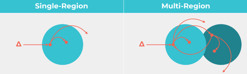
Both Single-Region and Multi-Regional Input-Output Analysis are valid methodologies. MRIO offers the advantage of providing a more robust and accurate picture of a local economy because most economies are not isolated to a single county.

An MRIO analysis allows you to keep the Multiplier identity of the core county (or region) while still being able to see how activity in the core region (where the Direct Effect takes place) touches other regions within a functional economy. Therefore, even if you were interested in the results in a single county, you could use MRIO if you wanted to capture feedback linkages to the core region from purchases your region made to those connected counties. However, in most cases this will not provide significant changes to your results.

3. Does the MRIO analysis provide a different net effect (or multiplier) than an analysis using only a single region?

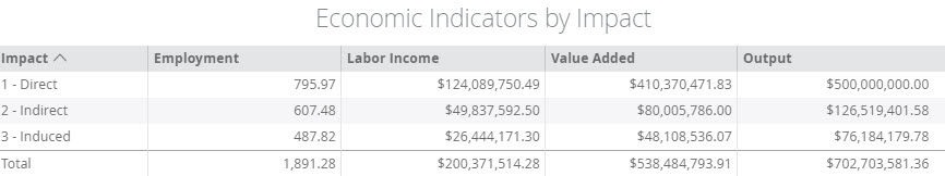
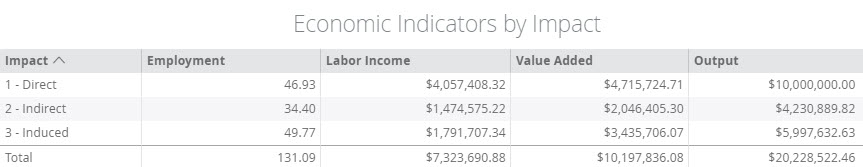
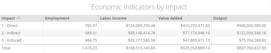
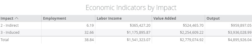
The only way to determine the Multipliers associated to an MRIO anlaysis is to calculate them by hand. We recommend exporting or copying/pasting your results to an Excel spreadsheet and summing the results to calculate the Multipliers using the base equation Total Effect/ Direct Effect. Please read this FAQ article to get more information about summing results from an MRIO and calculating the new Multipliers. The reason the Multipliers are different from single-region Multipliers is that we are capturing leakages to the linked regions that are lost from a single-region analysis. Therefore, there may be feedback from linked regions that will increase the effects in the core Study Area Region as well as the additional captured linkages represented in the linked Models.

The reason that this is a recommend analysis type is that it avoids the Aggregation Bias of aggregating Model regions. The state Multipliers will represent an average of all the firms in the state and their relationships for Output per Worker and Labor Income per worker. These can be drastically different from those in a smaller region, a cluster, or an MSA. Users are occasionally confused when the state actually has smaller values than the region where the Direct Effects occur; MRIO avoids this apparent anomaly that occurs when the supply of a commodity is concentrated in a single geography or a small group of geographies in a state, and thus demand at the state level increases without a substantial increase in supply. This happens in examples like Silicon Valley when considering tech Sectors.

4. Does MRIO provide region-specific effects from the aggregate analysis or completely different results from an aggregate region analysis?

MRIO Multipliers are unique and will be different from the aggregate region’s Multipliers (a region where all the files have been built into a single Model). The Multipliers in an aggregate Model are a weighted average of the region’s individual Industries and are thus subject to Aggregation Bias. These Multipliers are displayed in the Multipliers screen in the Explore menu. Conversely, MRIO Multipliers are unique to each set of linkages and must be calculated for each analysis as at no point are the regional Study Area Data information from the different areas combined.

5. Is MRIO effectively quantifying the ongoing chain of impacts?

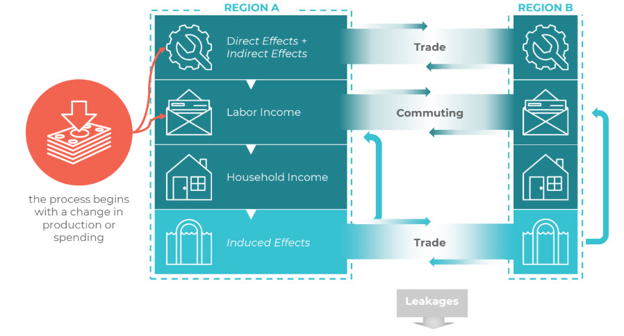
MRIO, in effect, extends the supply chain impacts into surrounding regions while still keeping the Multipliers for the core region intact and unique. Thus the rounds of additional impacts are extended to include feedback between all the linked regions until all purchasing dollars are leaked from the Indirect and Induced Effects.

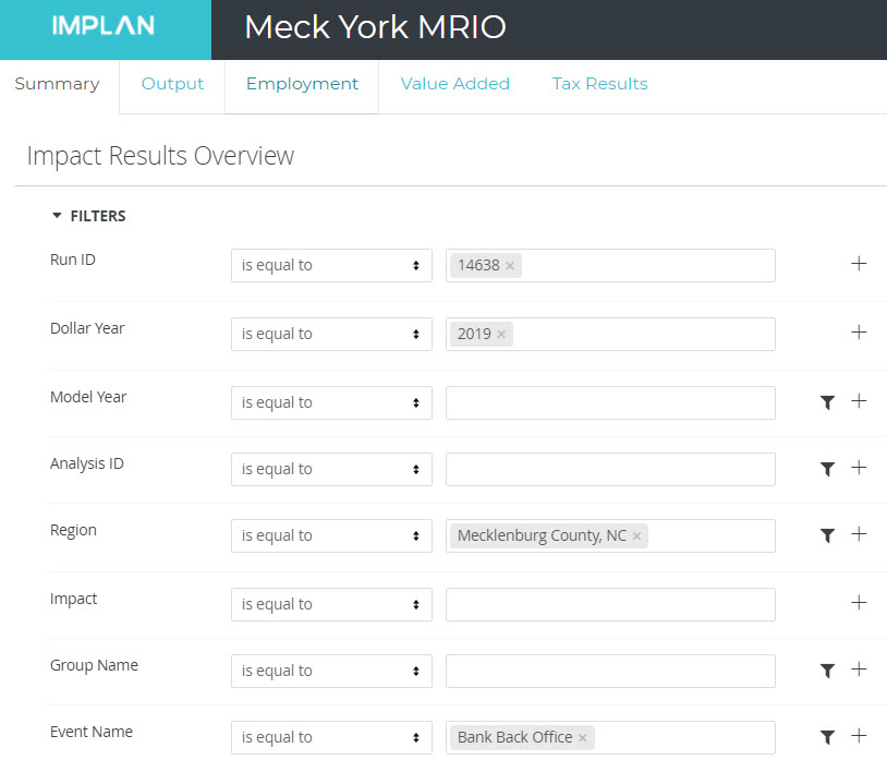
6. Are you able to aggregate the impact results of all models in the MRIO analysis into an “Impact Summary” within IMPLAN instead of exporting to Excel?

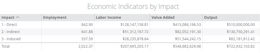
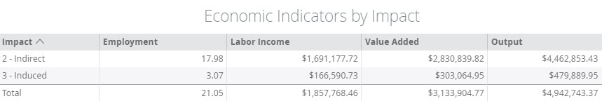
Not at this time. Impact results of all models in an MRIO analysis must be exported in order to sum the results. This allows you to individually quantify each regional impact and provides the flexibility to sum the regional impacts together to get a Total impact.

7. How do you aggregate the counties into “regions” and the “rest of state”?

You do this through the Model build process. When you build your Models you will select all the regions that you want incorporated into a single Model and then build that Model. This article provides additional information on aggregating Study Area regions in the Model building process.

8. How do you calculate a Multiplier for an MRIO Scenario?

You take the Total Effect (the sum of all the linked regions and the core) and divide this value by the Direct Effect for each factor. For additional information on how this is done, please see this Knowledge Base article.

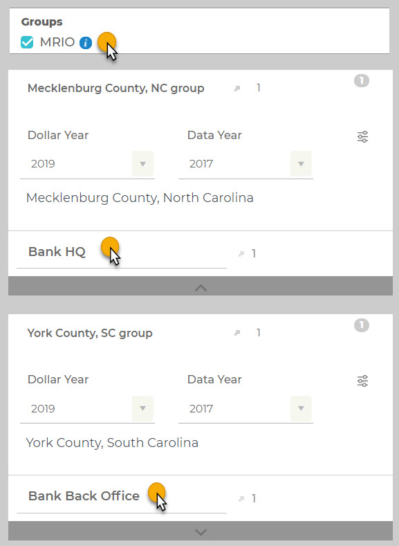
9. Do you need to enter the Activities into the linked models?

No, you only build the Activities in the region where your Direct Effect occurs. The Model linking process will calculate the impacts in the secondary Models. If you have Direct Effects in multiple regions, then you need to build a series of Models for each Direct Effect.

So let’s assume that we are dividing the state of CA into 4 regions: North California (NCA), North Central California (NCCA), South Central California (SCCA), and Southern California (SCA). If we only had impacts in NCA, we would need four Models: the NCA Model where Direct Effects are occurring and the three remaining Models we are linking to.

If we then have multiple Direct Effects in each region, we will need 16 Models: NCA, NCCA, SCCA, and SCA where NCA is the Direct Effect; NCA2, NCCA2, SCCA2, and SCA2 where NCCA is the Direct Effect; NCA3, NCCA3, SCCA3, and SCA3 where SCCA is the Direct Effect, and finally NCA4, NCCA4, SCCA4, and SCA4 where SCA is the Direct Effect. This prevents exponential explosion of the impacts from cross linking Models.

10. Where can I find information about the methodology IMPLAN uses to calculate the inter-regional flows of commodity?

We have a white paper in our downloads section that talks about the Gravity Model that lies behind the trade calculations. In addition, commodity flow data from the Bureau of Transportation is used as a Benchmark for the IMPLAN Trade Flows.

11. Where can I find additional documentation about MRIO?

We have some free documentation about setting up an MRIO on our website, and we also have available for purchase our Principles of Impact Analysis & IMPLAN Applications user manual. In addition, we can certainly assist you with analysis setup on our community pages.

12. Do ZIP code areas function similar to counties when conducting an MRIO Analysis?

MRIO is not viable for ZIP Codes at this time, as these data do not have Trade Flows. The level of data currently available at the ZIP Code level is too sparse for us to develop confident Trade Flows. However, there is a methodology for mock MRIO that can be done with ZIP Code level data and also Congressional Districts, which likewise do not have Trade Flow data.

Unfortunately, this means that if you add a ZIP Code or Congressional District level file to your county Model, the resulting Model will not be available for MRIO.

13. As an MRIO analysis links multiple study regions, how does IMPLAN determine each region’s share of the regional purchasing coefficient?

RPCs are calculated on the basis of the Gravity Trade Flow Model in the standard build (eRPC and Supply-Demand Pooling are also options you can exercise). The Trade Flows are also the basis of the MRIO analysis. This Trade Flow Model takes into account a variety of factors including the gravity of certain economies, impedences to trade, and cross-hauling.

14. How does MRIO take into account regions that border another country (Mexico)?

Unfortunately, IMPLAN does not have international trade flows at this time. Thus if imports are from outside the U.S., they are recognized by the Model as foreign imports/exports and are not tracked after they cross the national border. Therefore, international flows cannot be captured by the current Model. The Trade Flow data and MRIO are looking at domestic commodity flows.

Currently IMPLAN does not have data for most regions of Mexico, and therefore we are unable to develop Trade Flows at this time for North America; although, that is certainly something that we have in mind. It is important to note that the foreign imports/exports of commodities themselves are known, we just don’t have at this time flows to track where those foreign commodities are produced. This limitation is also exasperated by the limits of up-to-date raw data for international countries and their states and provinces.

15. How is MRIO’s ability to account for leakages an advantage over traditional Single-Region analyses?

Knowing where leakages go allows you to account for them. In a single region analysis, leakages are just lost. Thus, importing 75% of commodity A means that 75% of the value of commodity A is lost in the first round of the impact analysis. But in reality, that 75% goes to some economy somewhere. MRIO allows you to see if and how your impact in the core region is affecting surrounding regions. Thus if you can buy an additional 5% from region R2, then you can now account for (in region R2’s results) that 5% and demonstrate both where it goes and that it results from your change to the economy. Likewise, if that 5% in region R2 is spent on a commodity that can now be imported from region R1, you capture that additional round of impact.

MRIO: Multi-Regional Input-Output Analysis When More Than One Region Includes Direct Impacts

INTRODUCTION:

Sometimes you may have more complicated analyses that you want to run.  Let’s say the bank opening up in Mecklenburg County, NC from the Introduction to MRIO article will also be opening up a smaller office in York County, SC.  This can be modeled with Multi-Regional Input-Output (MRIO) analysis to see what the effect of each project will have on the two counties together and separately.


THE PROCESS:

STEP 1 – SETTING UP THE EVENT

In our example, the new bank HQ will be opening in Mecklenburg County, NC with $500M in projected Output.  Taking this one step further, the bank plans to open a smaller back office facility in York County, SC with a projected $10M in Output.  As with the HQ example, this office will closely resemble a financial institution and not support services, so Sector 433 – Monetary authorities and depository credit intermediation was chosen as the sector.

First, on the Regions screen, select both Mecklenburg County, NC and York County, SC.  Click Create Impact.  

Create an Industry Output event in Sector 433 – Monetary authorities and depository credit intermediation for $500M.  Save the Event and drag it into the Mecklenburg County group on the right side of the screen.  

Create a second Industry Output event in Sector 433 – Monetary authorities and depository credit intermediation for $10M.  Save the Event with a different name than the first so that it can be identified later. Drag it into the York County group on the right side of the screen.  Each Region has its own Event associated with it.

Ensure that the MRIO checkbox at the top of the screen is checked.

MRIO_2_Direct_-_Regions.jpg

Click Run.  When using MRIO, the software will take a little longer than a standard analysis.  Grab a cup of coffee and when the analysis is complete, click View Results.


STEP 2 – VIEWING THE RESULTS

When you look at the Results screen, you see the Total Direct Output of $510M; $500M in Mecklenburg for the HQ and $10M in York for the back office.  Together, they have an indirect effect of $131M and an induced effect of $82M, for a total economic impact of $723M. These results include the impacts of the HQ and back office locations on both Mecklenburg County, NC and York County, SC.

Mecklenburg County & York County Impact – HQ and Back Office

MRIO_2_Direct_-_M_Y_HQ_BO.jpg

Unlike when there is only one region with an Event, now there are two options for Filtering the results.  We can see how the new back office operations (located in York County, SC) will spur economic activity in Mecklenburg County, NC. In the Region box, choose Mecklenburg and in the Event Name box choose “Bank Back Office.” Hit the run button on the right.

MRIO_2_Direct_-_Filter.jpg

Notice that there is no Direct impact.  You do see a total Output impact of almost $5M. This is money that will flow into Mecklenburg County because of the $10M in bank back office operations in neighboring York County.

Mecklenburg County Impact – Back Office

MRIO_2_Direct_-_M_BO.jpg

By only filtering the Region for Mecklenburg, we will see the effect of the HQ and the back office on the county.  This shows us the Direct Output of $500M for the HQ, but not the $10M in Direct Output for the back office.


Mecklenburg County Impact – HQ and Back Office

MRIO_2_Direct_-_M_HQ_BO.jpg 

If the Region is filtered by York County, you will see the effect of the HQ and the back office on the county.  This shows us the Direct Output of $10M for the back office, but not the $500M in Direct Output for the HQ.

York County Impact – HQ and Back Office

MRIO_2_Direct_-_Y_HQ_BO.jpg

If you add the Economic Indicators from Mecklenburg and York counties, you will get the total Output impact of $723M seen before the Filter was applied.


RELATED TOPICS:

Introduction to Multi-Regional Input-Output (MRIO)

Considerations when using MRIO

Size of Your Impact – Questions & Concerns about Small vs. Large Study Regions & MRIO

Multi-Regional Input-Output (MRIO) Analysis FAQ

MRIO: Size of Your Impact – Questions & Concerns about Small vs. Large Study Regions

Introduction

Larger study areas tend to reflect larger impacts, because larger geographies typically capture more production as ‘local’ and are subject to less in-commuting. However, analysts are occasionally surprised to find that the economy of a smaller subset region, such as a county, reflects a greater Indirect and Induced impact than that of the larger aggregate region (i.e., the state). Although not exhaustive, this article does highlight the most common reasons for such an occurrence. One easy way to avoid these issues, if you are using IMPLAN Pro, is to use the MRIO methodology.

Detail Information

Why does this occur? How can a smaller region have greater Indirect and Induced Effects than it has when you include surrounding geographies?

Typically larger Indirect and Induced impacts in a smaller subset region are the result of areas of high production surrounded by more rural regions. This creates a situation where we see only a small bump in production between the smaller geography and the larger one, but a significant increase in demand. This change can be economy wide, or it could be related to a specific commodity as a result of regional specialization or clustering. In these areas, the supply relative to demand is much higher in the smaller region than in the larger region (i.e., the RPCs for what is regionally available in the smaller region exceeds that of the larger region). Therefore, the larger geography sees a much larger increase in demand for the products produced in the smaller geography but does not substantially increase the supply available to meet that demand. Wyoming is a classic example of this type of activity because there are few regions of supply and a vast state of demand.

These same principles can apply in regards to Labor Income and Value Added because the regions of greater production often pay higher wages per worker and may pay higher taxes (or be subject to additional taxes such as city taxes not collected in the rest of the county). Since Value Added = Labor Income + Other Property Type Income + Taxes on Production & Imports Net Subsidies, if either or both income and taxes are higher, or if profits are higher in the core region, “upside down” effects, where the results are higher in the smaller region (county) than in the larger region (state), may be generated.

When using Employment to estimate the impact of an Industry an additional caveat arises because a difference in Output per Worker can generate significantly variant Output estimates. If the Output estimate in the smaller region is substantially larger the Output estimate in the larger region, this can result in Indirect impacts in smaller subset regions being larger than in the aggregate regions. Production areas with a greater Output per Worker than the larger surrounding area may reflect a larger impact than the aggregated region as a whole.

Usage

Typically, when impacting a larger study region, the results will follow the “normal” pattern of the Indirect and Induced producing large impacts. However it is still advisable to match the Event values in the larger region to those of the county, as this results in a consistent estimate of the Direct Effects.

This same technique also works for adjusting these smaller regions that produce higher impacts than their larger aggregate. Modify the Event in the larger region to match the Event in the smaller region (e.g., same output-per-worker, same labor income per worker) will typically resolve this issue.

However, if sufficient data is availalbe, IMPLAN recommends MRIO (Multi Regional Input Output) rather than direct comparisons of the aggregate state file to a county subset. Before IMPLAN had MRIO capability, analysts were forced to:

  1. Choose the small region where the actual direct impact occurs but lose much of the indirect and induced impact to leakage.
  2. Choose a larger region to capture those leaked impacts, but now the impact location is less precisely defined.

This is no longer necessary with the ability to use MRIO. Now the smaller region can be chosen for the Direct impact while still affording analyst the ability to see the impact on the neighboring regions (and those regions’ feedback effects back on the smaller region). MRIO also allows for each region to keep it’s unique identity and for you to be able to see how the impacts in the core sub-region and the larger aggregate region occur.

MRIO: Considerations when using Multi-Regional Input-Output Analysis

Building your Economic Analysis with multiple regions utilizing MRIO (Multi Regional Input/Output) enhances your study. That is, MRIO demonstrates how an impact in your Study Area disperses into other regions and allows you to see how these effects in surrounding areas create additional local effects. For each Industry, MRIO not only tracks the imports from every other Industry, but also where those Imports are coming from. Each region’s production relationships and local purchasing abilities remain distinct. While the MRIO model will still lose the same dollar amounts as imports within the defined local area, these impacts will be visible in the linked models. Additionally, MRIO can look back to the original regional model and capture expenditures made in auxiliary regions that will impact the original local model, capturing impacts that are completely untraceable without MRIO capacity.

In the past, other MRIO methodologies have been attempted as the best available option, but were not true MRIOs. The following considerations demonstrate the problems that may be caused if MRIO is not utilized.

1. To create a comparable analyses, the Sector of the larger Model file will need to be modified to demonstrate local relationships.

The Industry relationships at the state or U.S. level would need to be forced to be the same as the Industry at the local level. This means that the US or state level Model’s Industry must have the same Output Per Worker, Earnings Per Worker, etc as the local Industry. This is the only way to attempt to adequately represent how the local Industry is making its purchases relative to the larger Model. However, this is just an approximation; the actual relationships with which the larger region would purchase products are unknown in this instance.

For additional information on performing this type of analysis click here.

 2. The local region and the larger region will have differences in internalized Imports, which cannot be adjusted.

The ability of a product to be sourced locally may be significantly higher at the state or U.S. level than at the local level (or in some rare instances, they may be lower). This in turn will impact the Multipliers of the model.

Additionally because there is no way to separate out the local region’s economy in standard analysis, the two studies and impacts must be considered as two completely independent impacts. Since the larger geographic region may include local purchases to what would be considered Imports in the regional Model, there may also be increased impacts resulting in the regional portion of the Model. Therefore even with the modifications in Consideration 1, the regional impacts which will accurately represent the local region cannot just be “subtracted” from the larger area.

MRIO: Introduction to Multi-Regional Input-Output Analysis

INTRODUCTION:

Multi-Regional Input-Output (MRIO) analysis makes it possible to track how an impact on any of the 536 IMPLAN sectors in a Study Area region affect the production of all 536 sectors and household spending in any other region in the US (state to state, county to county, zip code to zip code, county to multi-county, county to state, etc). Now you can demonstrate how an impact in your Study Area disperses into other regions and see how these effects in surrounding areas create additional local effects.  

MRIO_-_Region_A___B.jpg

Let’s say a new bank is opening up a HQ in your county and the state gave them a huge tax incentive to locate there.  Using MRIO you can show each county how the bank locating in one county will also impact their county, thus making it a valuable investment of state tax dollars.

We live in regional ecosystems and when running an impact analysis you can see how much money leaks out of your city through trade and commuting.  Using MRIO you can see where some of that leakage ends up – supporting other cities across the county or state. 

There are many reasons you may want to consider using MRIO.

  • To improve the methodology of your study
  • To improve the regional specificity and limit aggregation bias
  • To examine the interconnectedness of multiple regions
  • To track leakages from a study region and determining the impacts they create in other regions


HOW MRIO WORKS:

MRIO expands backward supply linkages beyond the boundaries of a single-region Study Area.  MRIO analyses utilize interregional commodity trade and commuting flows to quantify the demand changes across many regions stemming from a change in production and/or income in another region. This powerful analytical method allows analysts to go beyond a single study region, measuring the economic interdependence of regions.

In an MRIO analysis, the Direct Effect in one region, Region A, can trigger Indirect and Induced Effects in linked regions, capturing some of what would have been a leakage in a traditional I-O model.

Let’s say a new firm is opening in Region A. Some of the construction inputs may be produced in linked Region B and are imported into Region A. Through this trade there is a production change in Region B that triggers a whole new change of spending in Region B. If the construction materials produced in Region B require an input produced back in Region A, thus creating a new branch of backward linkages in Region A. 

As always jobs supported by the new production and the affected supply chain earn income, but potentially workers in Region A will live in Region B and visa versa.  As dollars trickle to household spending, there is likely trade between the regions in the supply chain. For example, restaurants in region A frequented by the workers that reside in region A may buy produce from a farmer in Region B. The income earned by workers on the farm would trigger a new chain of labor income. Some of the farm workers may live in Region A, so household spending cycles through both regions. 

Trade and commuting dollars bounce between regions until they funnel through the rest of the economy or are leaked out as imports to other regions or through profits and taxes. 

MRIO_-_How_it_Works.jpg

THE PROCESS:

STEP 1 – SETTING UP THE REGIONS

Charlotte, NC is the second largest financial center in the US. For this example, let’s say a new bank will be opening and you want to see the effect not only in Mecklenburg County, NC, but also in neighboring York County, SC. 

First, on the Regions screen, select both Mecklenburg County, NC and York County, SC.  Click Create Impact. In some cases you may want to create Combined Regions to build a clustered surrounding area. For example, we want to additionally see the effect on the surrounding Charlotte MSA within North Carolina in which case we could select all the Counties in the Charlotte MSA in NC except for Mecklenburg County and Combine these Regions to form 1 new Region. We must exclude Mecklenburg if we are including it as its own Region, otherwise the effects in Mecklenburg will be double-counted in our MRIO Analysis. Combining Regions is beneficial especially within an MRIO Analysis because it will reduce the analysis run time.  

MRIO_2_Direct_-_Checkbox.jpg

STEP 2 – SETTING UP THE EVENT

Create an Industry Output event in Sector 433 – Monetary authorities and depository credit intermediation for $500M.  This sector was chosen because the primary function of the HQ in this instance more resembles a financial institution than the traditional HQ functionality.  If the firm was following a traditional HQ, then Sector 461 – Management of companies and enterprises, would be the correct choice. For more information, visit the US Census Bureau.

Save the Event and drag it into the Mecklenburg County group on the right side of the screen.  No event will be added to the York County group as the bank will operate in Mecklenburg.  

Ensure that the MRIO checkbox at the top of the screen is checked.

MRIO_-_Checkbox.jpg

Click Run.  When the analysis is complete, click View Results.

STEP 3 – VIEWING THE RESULTS

When you look at the Results screen, you see the Total Direct Output of $500M which has an indirect effect of $123M and an induced effect of $80M, for a total economic impact of $703M.  These results include both the impacts on Mecklenburg County, NC and York County, SC.

Mecklenburg County & York County Impact

MRIO_-MY.jpg


In order to see how this new bank will affect its home county of Mecklenburg, we need to Filter our results.  In the Region box, choose Mecklenburg and then hit the run button on the right.

MRIO_-_Filter.jpg

The Total Direct Output remains $500M, because the bank will be located within Mecklenburg.  However, the indirect and induced effects are only showing the activity within this county, so you see a total of $698M in Output impact.


Mecklenburg County Impact

MRIO_-_M.jpg

If you change the Region Filter to York County, SC and hit run, you see the impact that the new bank in NC will have on York County, SC.  Notice that there is no Direct impact. You do see a total Output impact of almost $5M. This is money that will flow into York County because of the bank operations in neighboring Mecklenburg.


York County Impact

MRIO_-_Y.jpg

If you add the Economic Indicators from Mecklenburg and York counties, you will get the total Output impact of $703M seen before the Filter was applied.


USEFUL TIPS:

MRIO works best with up to seven regions.  When possible, create aggregated regions to examine the effects on the other areas.  For example, to look at the economic impact on Mecklenburg County and the remainder of North Carolina, create a region of the remaining 99 counties.  

Every region has a unique set of commuter rates, trade flows, and region specific identities (Output per worker, Intermediate Expenditures to Value Added, etc.)  Therefore, you will see different results if you run an impact on a combined Region A + Region B versus an MRIO on Region A and Region B.


CASE STUDY:

Regional Fission: How MSU Accelerated Their Research Facility Funding Using MRIO


WEBINAR:

Multi-Regional Input-Output: A Primer, How-To Guide, and Best Practices 


RELATED TOPICS:

Multi-Regional Input-Output (MRIO): When More Than One Region Includes Direct Impacts

Considerations when using MRIO

Size of Your Impact – Questions & Concerns about Small vs. Large Study Regions & MRIO

Multi-Regional Input-Output (MRIO) Analysis FAQ

Generation and Interpretation of IMPLAN’s Tax Impact Report

Generation and Interpretation of IMPLAN’s Tax Impact Report  


FILTERING:

To filter by Direct, Indirect, and Induced taxes in IMPLAN, simply open the Filter window and click into the “Impact” Filter. This will provide you the option of “Direct”, “Indirect”, “Induced”. Making a selection and clicking “Run” will apply the filter and only show the Tax Results as specified. if no selection is made, you are viewing total Tax Results. 


tax_filter.png


TAX IMPACT DETAILS:

The table below clarifies the underlying level of detail of all line items in an IMPLAN tax impact report. In principle, the tax impact report captures all tax revenue in the study area across all levels of government that exist in that study area for the specific industries and institutions affected by an event or group of events. The underlying data that support the tax impact report, however, do not embody that much detail.

For example, IMPLAN does not have systematic reports of state government tax revenue by county; IMPLAN has same-year state government tax revenue by state and must allocate that to counties based on proxy information (we do have county-level data for some states, and use this to build a model for the allocation process).  Also, IMPLAN obtains detailed TOPI data by geography (even for each city within a county), but does not have any industry detail about the specific TOPI line item. A third note: for the data by city, we often must aggregate that to the county level, so that a model of two cities in the same county will have the same implied effective tax rates. In other words, city-specific data will be used, but averaged across all cities within a county.

Please note that all line items are controlled to nationwide, current-year controls estimated by the Bureau of Economic Analysis (BEA) in the National Income and Product Accounts (NIPAs) with no industry resolution and two level-of-government distinctions, Federal and State & Local. For example, the NIPAs might give a value of $15 billion in State & Local income tax in 2017, which would be reflected in the 2017 IMPLAN data.

Industrial and geographic resolution are reported at their maxima and nest more aggregate levels. For example, if IMPLAN has raw data on property tax at the county level, that implies we also have state-level data.

Timeliness lags are reported vis-à-vis the dataset year. For example, a 1 year lag for 2017 IMPLAN data means that the underlying data have a reference year of 2016. Timeliness is especially relevant for knowing whether changes in tax laws or economic conditions are reflected in the IMPLAN dataset.

The table below does not report the combined State & Local level of government, since (other than nationally in the NIPAs as explained above) IMPLAN does not collect any data at this level; it’s simply an aggregate for legacy and convenience purposes.

Level of Government Tax Impact Item Maximum Industry Resolution of Underlying Data Maximum Geographic Resolution of Underlying Data Timeliness of Underlying Data

City/Special District

TOPI: Property Tax

TOPI aggregate at BEA sectoring (approximately 80 sectors).

TOPI detail has no industry resolution.

County level

1-2 years lag

City/Special District

TOPI: Motor Vehicle License

TOPI aggregate at BEA sectoring (approximately 80 sectors).

TOPI detail has no industry resolution.

County level

1-2 years lag

City/Special District

TOPI: Severance Tax

TOPI aggregate at BEA sectoring (approximately 80 sectors).

TOPI detail has no industry resolution.

County level

1-2 years lag

City/Special District

TOPI: Other Taxes

TOPI aggregate at BEA sectoring (approximately 80 sectors).

TOPI detail has no industry resolution.

County level

1-2 years lag

City/Special District

TOPI: Special Assessments

TOPI aggregate at BEA sectoring (approximately 80 sectors).

TOPI detail has no industry resolution.

County level

1-2 years lag

City/Special District

Personal Tax: Income Tax

n/a

County level

1-2 years lag

City/Special District

Corporate Profits Tax

None

County level

1-2 years lag

City/Special District

Personal Tax: Motor Vehicle License

n/a

County level

1-2 years lag

City/Special District

Personal Tax: Property Tax

n/a

County level

1-2 years lag

City/Special District

Personal Tax: Other Tax

n/a

County level

1-2 years lag

County

TOPI: Property Tax

TOPI aggregate at BEA sectoring (approximately 80 sectors).

TOPI detail has no industry resolution.

County level

1-2 years lag

County

TOPI: Motor Vehicle License

TOPI aggregate at BEA sectoring (approximately 80 sectors).

TOPI detail has no industry resolution.

County level

1-2 years lag

County

TOPI: Severance Tax

TOPI aggregate at BEA sectoring (approximately 80 sectors).

TOPI detail has no industry resolution.

County level

1-2 years lag

County

TOPI: Other Taxes

TOPI aggregate at BEA sectoring (approximately 80 sectors).

TOPI detail has no industry resolution.

County level

1-2 years lag

County

TOPI: Special Assessments

TOPI aggregate at BEA sectoring (approximately 80 sectors).

TOPI detail has no industry resolution.

County level

1-2 years lag

County

Personal Tax: Income Tax

n/a

County level

1-2 years lag

County

Corporate Profits Tax

None

County level

1-2 years lag

County

Personal Tax: Motor Vehicle License

n/a

County level

1-2 years lag

County

Personal Tax: Property Tax

n/a

County level

1-2 years lag

County

Personal Tax: Other Tax

n/a

County level

1-2 years lag

State

TOPI: Property Tax

TOPI aggregate at BEA sectoring (approximately 80 sectors).

TOPI detail has no industry resolution.

State level

0 years lag

State

TOPI: Motor Vehicle License

TOPI aggregate at BEA sectoring (approximately 80 sectors).

TOPI detail has no industry resolution.

State level

0 years lag

State

TOPI: Severance Tax

TOPI aggregate at BEA sectoring (approximately 80 sectors).

TOPI detail has no industry resolution.

State level

0 years lag

State

TOPI: Other Taxes

TOPI aggregate at BEA sectoring (approximately 80 sectors).

TOPI detail has no industry resolution.

State level

0 years lag

State

TOPI: Special Assessments

TOPI aggregate at BEA sectoring (approximately 80 sectors).

TOPI detail has no industry resolution.

State level

0 years lag

State

Personal Tax: Income Tax

n/a

State level

0 years lag

State

Corporate Profits Tax

None

State level

0 years lag

State

Personal Tax: Motor Vehicle License

n/a

State level

0 years lag

State

Personal Tax: Property Tax

n/a

State level

0 years lag

State

Personal Tax: Other Tax

n/a

State level

0 years lag

Federal

Social Insurance Tax- Employee Contribution

None

State level

0 years lag

Federal

Social Insurance Tax- Employer Contribution

None

State level

0 years lag

Federal

TOPI: Excise Taxes

TOPI aggregate at BEA sectoring (approximately 80 sectors).

TOPI detail has no industry resolution.

National level

0 years lag

Federal

TOPI: Custom Duty

TOPI aggregate at BEA sectoring (approximately 80 sectors).

TOPI detail has no industry resolution.

National level

0 years lag

Federal

Corporate Profits Tax

None

National level

0 years lag

Federal

Personal Tax: Income Tax

n/a

National level

0 years lag

Federal

Personal Tax: Estate and Gift Tax

n/a

n/a

n/a


Updated September 3, 2019

Compensation Adjustment in New IMPLAN to Account for Known In-Commuting Rate

To view the commuting data for your region, go to Explore > Social Accounts > IxC Social Accounting Matrix. If the Employee Compensation column makes a payment to the Domestic and/or Foreign Trade row, then there is in-commuting into the region (income earned by workers who work in the area and live outside the area). The ratio of Domestic plus Foreign trade value divided by the Employee Compensation column total gives you an estimate of the in-commuting rate. This rate is referred to as the “samCR” below. If the cell is empty, then there is no in-commuting into the region. 

commuting.PNG

The equation below allows you to adjust IMPLAN’s estimated regional commuting rate to your known regional commuting rate.


newEC = EC*[(1-userCR)/(1-samCR)]

where:

EC = original, unmodified employee compensation

userCR = your known commuting rate

samCR = commuting rate reported in the SAM

newEC = the EC value you want to use when running the analysis


For example, if the SAM shows that the average in-commuting rate in your region is 10% but you know that for your industry it is 20%, then: new EC = $1,000,000*(0.8/0.9) = $1,000,000*(0.88888) = $888,888.

After the analysis has been run, add the difference (EC – newEC) back to your direct EC effect since by definition EC occurs at the site of employment. Since EC is a component of Value Added, you should update the calculation of Value Added to include the difference. Because payroll taxes (social insurance taxes) are paid at the site of employment, the direct effect payroll taxes in your tax results will also need to be revised to their pre-EC adjustment levels. Create a separate activity, duplicate your event but use your EC value that has not been adjusted for commuting, and perform the analysis in a new scenario. Use the resulting direct effect EC payments to social insurance as replacement values for your adjusted EC analysis and re-sum the direct effect and total effect tax impact tables. This way you correctly account for the in-commuters’ direct effect, but you have also made sure that they did not generate any further local impact.

Local Purchase Percentage (LPP) & Regional Purchasing Coefficients (RPC)

INTRODUCTION:

Local Purchase Percentage (LPP) and Regional Purchasing Coefficients (RPC) are two of the most frequently misused and misunderstood fields in IMPLAN. This article describes what these concepts mean and when they should be changed from the default settings.


LPP IN INDUSTRY EVENTS:

Local Purchasing Percentages (LPP) indicates to the software how much the Event impact affects the local Region and should be applied to the Multipliers. The key thing to remember when considering Local Purchase Percentage is that the LPP modifies only the Event values, and it does this before those values are applied to the Multipliers.  If we have properly defined the Region, then in most circumstances all of the Industry Production we are modeling occurs within our selected geography and thus LPP should be 100%. When LPP is less than 100%, the remaining portion (or 1-LPP) is then assumed to be affecting a different Region. The portion happening outside the Region of your analysis does not create any local effect.  

Local Purchase Percentage describes the amount of the Direct Effect that is taking place within the Region. For example, if we are constructing a building in a county, all the construction activity takes place in that county, even if all the laborers and the requirements for the building are not sourced in the county, so LPP should be 100%. Likewise, if the operations of new or expanded business are occurring entirely inside our county, even if their employment or materials are sourced elsewhere the LPP should be 100% because the business operations themselves are local.

Changing LPP from 100% in an Industry Event is infrequently appropriate, but one classic example is that of airline ticket purchase. Although $850 may be spent on a ticket, the cost associated with that ticket is divided between the point of origin and destination. Therefore the total budget spent on airline tickets for a business trip may be $850, but the local airport only incurs half of the associated cost.

    • A Local Purchase Percentage of 100% means that all of the Industry Production is occurring within the Model region and all the Employment occurs within the Model region.
    • By definition in Input-Output, Employment is at the site of work, so all employees, regardless of where they live, are counted as employment for the region if they work at a site within the region.
    • Considerations of where an employee lives are taken into account by means of the Employment Compensation and Proprietor Income fields. (Please see the Related Articles section on the topic of Commuting).


LPP IN COMMODITY OUTPUT EVENTS:

Again, Local Purchasing Percentages (LPP) indicate to the software how much the Event impact affects the local Region and should be applied to the Multipliers. The key thing to remember when considering Local Purchase Percentage is that the LPP modifies only the Event values, and it does this before those values are applied to the Multipliers. When LPP is less than 100%, the remaining portion (or 1-LPP) is then assumed to be effecting a different Region. The portion happening outside the Region of your analysis does not create any local effect. 

Commodity Output Events are typically used to model a purchase or purchases of a certain Commodity. When the Commodity is known to be produced locally in the Region, leaving LPP at 100% is appropriate. It is common that the location of production of a purchased Commodity is unknown, in which case you can let IMPLAN determine what portion of the production may affect the local Region by selecting the SAM Checkbox next to the LPP field in the Advanced Menu. 


LPP IN SPENDING PATTERN EVENTS:

Industry and Institutional Spending Patterns start the analysis, not from the standpoint of the sales or Employment of the Industry or Institution, but instead from the budgetary purchases made by the local organization.

LPP in an Industry or Institutional Spending Pattern tells the software what portion of the line item Commodity was purchased locally and therefore affects the local Region.  When LPP is less than 100%, the remaining portion (or 1-LPP) is then assumed to be effecting a different Region. The portion happening outside the Region of your analysis does not create any local effect. 

Unlike the Industry or Institution itself, we typically cannot say where the production, transport, and wholesaling of the items purchased by our target organization was sourced, and we would not want to assume that these are local purchases. Since this methodology, unlike an Industry Event or Commodity Event, starts not from the Industry or Commodity itself, but from the first round of Intermediate Expenditures, the LPP on these purchases needs to reflect local availability. Thus the LPP is by default set to the SAM Model Value. You would only want to change the LPP on the Commodities within a Spending Pattern if you had information on where the Commodity was produced. 


LPP EXAMPLE:

To help envision this more clearly, we can take a look at a quick example to see how the software uses Local Purchase Percentage.

    • An Event for Sector 12 Dairy Farming has shows the following:
      • Industry Sales: $1,000,000
      • Employment: 6
    • If Local Purchase Percentage is set to 50% then the Direct Effects will be $500,000 of Output and 3 jobs. Why?
      • To calculate, the software first multiplies the Industry Sales value by the Local Purchase Percentage ($1,000,000 * 0.50 = $500,000)
      • The software then recalculates the Employment and Labor Income based on this adjusted Industry Sales value, which is half of the entered value and thus generates half the Employment and Labor Income.
      • Deflators are applied to adjust the entered value down to the year of the data set. This makes the dollar values used to calculate the Multipliers equivalent to the entered dollar values.
      • The resultant value is applied to the Multipliers to determine the Indirect and Induced Effects.
      • Thus, the LPP does not provide any information about any of the items purchased by the Sector in the Event field. Regional availability of Intermediate Expenditures and Indirect Effects are determined by the Regional Purchasing Coefficient.


RPC DETAILS:

A Regional Purchasing Coefficient (RPC) is the percent of Total Demand that is met by Local Supply. In more detail, it is the proportion of the Total Demand for a Commodity, by all users in the Region, that is supplied by producers located within the Region. The RPC is the value used when LPP is set to the SAM Model Value.

For example, if the RPC for the Commodity fish is 0.8, then 80% of the demand by local fish processors, fish wholesalers, and other fish consumers are met by local fish producers. Conversely, 20% (1.0-RPC) of the demand for fish is satisfied by imports. 

The RPC value is derived from the Trade Flow Model that looks at the movement of Commodities domestically and known rates, by Commodity, for foreign trade. The RPC value tells us, for every Commodity we purchase, how much of our total requirement for that Commodity is obtained from local sources according to the Region and Year of the Data Set. This value is built into the Multipliers, so you never need to make any adjustments to your Event to account for locality of the goods and services required for your production.

The RPC does not assume that all local production goes to local demand (i.e., Regional Supply Coefficient (RSC) may not be 100%). Each Commodity’s RPC can be found in Regions Overview > Social Accounts > Reports > Commodity Summary, Average RPC column.  Values for the RPC are between 0 and 1. Also, the LPP is equal to RPC only when the regional availability of the product is unknown. RPC values cannot be changed in app.implan.com.


RELATED TOPICS:

Commuting

Margining: When the Item Being Purchased Is Known

Margining: When the Item Being Purchased in Unknown

The New IMPLAN: What’s so New About It?

CONTENTS

The contents of this article are outlined below. If you already know what you’re looking for, click on a link to advance to a specific section!

1. No more time wasted setting up
2. Faster calculations
3. More fluid workflows
4. Multi-tab functionality
5. A few labels…
6. Easier-to-edit industry spending patterns
7. Better SAMs
8. Multi-angular MRIO
 

INTRODUCTION

From Quesnay’s Tableau économique to Leontief’s Nobel Prize-winning work on modern input-output analysis, impact modeling has a fascinating history. In the nearly 50 years since Leontief, I/O’s application has evolved in both universality and convenience to a degree which few could ever have imagined. Today, coupling improvements in analytical methodology with innovative technologies looks to propel economic impact modeling to its greatest heights yet. And the new IMPLAN hopes to be the primary means by which it reaches them. 

WHY IS THERE A NEW VERSION OF IMPLAN?

The honest answer is…we knew we could do better for you. We value the loyalty, support, and trust that you, our users, have given us over the past 25+ years. If we hope to continue receiving them from you over the next 25+ years, we need to earn them. So, we’ve been hard at work improving our data, revolutionizing our tool, and strengthening our organization to better serve your economic needs.

The new IMPLAN is the culmination of nearly 3 years of work. We’ve been revisiting our legacy tools, listening carefully to (and actively engaging with!) the economics community, and then employing the latest in computing power to meet even its toughest demands. We’re really excited about what we’ve built and we think you will be too. 

The new platform is designed to alleviate the day-to-day challenges of both economists and non-economist alike. From public policymakers to institutional researchers to economic scholars and beyond, those who rely on input-output modeling to shape our understanding of communities both large and small can now do so more conveniently than ever before. In fact, understanding theses groups’ creative uses of IMPLAN was pivotal in helping us develop a tool which now provides even more ways to access, review, and interpret both regional economic data and powerful impact results.

Plus, with a whole bunch of enhanced features, doing all of those classic things you’ve always done with IMPLAN is not only still possible, it’s easier. You don’t have to click on confusing buttons anymore. You don’t have to navigate overcomplicated screens anymore. And you don’t have to execute procedures in a strict and unforgiving order anymore. The new IMPLAN’s flexibility and ease-of-use is unrivaled by any previous iteration you may be familiar with.

Seriously, this version is a game changer.

HOW IS IT BETTER THAN THE VERSION I USE?

1. NO MORE TIME WASTED SETTING UP

Most single geography “Models” you used to spend valuable time building ad hoc are now simply saved as pre-built Regions. So, instead of going through the motions of opening a saved Model or rebuilding one from scratch because you deleted it, now you just select your study’s Region from a dropdown menu. That’s it. And if you edit it, customize it, rename it, save it, come back to it later, edit it again… Whatever. Literally a brand-new, untouched version of that very same Region is always available to you in that little dropdown menu. No more Model-building responsibilities on your shoulders. IMPLAN’s already done it for you—even before you’ve started.

2. FASTER CALCULATIONS

The new IMPLAN’s analysis engine relies on Amazon Web Services (AWS) to do all its dense, heavyweight computing in the cloud. So, this version has enough muscle under the hood to match the demands of even the most sizable IMPLAN projects. This all but eliminates any “wait time” for complex calculations to finish (…sorry to anyone who’s used those procedural interruptions as an excuse to take a break in the past!).

3. MORE FLUID WORKFLOWS

Jump into an analysis from wherever is most natural to you. Know what real-life impact you want to model but not sure exactly what geography you want to study? No problem. Tell IMPLAN everything you know about the impact first, then come back and select a Region later. Know which regional economy you want to analyze but not sure of all the details of your real-life impact quite yet? That’s cool too. Tell IMPLAN which geography you want to study first, then come back and create an Event later.

With IMPLAN’s new project-based workflow, you can start anywhere. Duplicate Events, Regions, and more, and then mix-and-match them quickly and easily without having to jump through a bunch of hoops to set it all back up again. Honestly, you can run 10 complete analyses and be reviewing their results with the same amount of energy it used to take to run just one.

4. MULTI-TAB FUNCTIONALITY

The new IMPLAN isn’t just more convenient to start using, faster in calculating results, and more practical to operate—it’s also categorically more comfortable to interact with. For instance, the new IMPLAN lets you spread your work out across multiple tabs inside your internet browser while you’re working. Within the confines of even a single Project, you can open three different tabs in your internet browser and separate the REGIONS, IMPACTS, and RESULTS screens across them in order to look at all your study’s components at the same time. You don’t have to keep going back and forth between screens to clarify your Region, check your inputs, or confirm your outputs anymore. Apart, IMPLAN and the internet were already awesome. Now they’re awesome together.

WHAT ARE THE BIGGEST DIFFERENCES WITH THIS VERSION?

5. A FEW LABELS…

Some of the new IMPLAN’s most obvious changes pertain simply to how things are labeled or referred to within the tool. The biggest of these changes is with regard to how the tool now refers to the different kinds of impact studies IMPLAN users can run. 

Table_1__the_new_IMPLAN_article_.png

Specifically, what used to be referred to as an “Activity Type” is now simply called an Event Type. While the name may have changed, that’s all that’s changed. Defining an Event Type works exactly the same way as selecting an “Activity Type” always did; simply pick the one that best describes the kind of impact study you’re performing.

So… Why the change? Fair question. The reason is because while “Activities” and “Events” used to exist as two separate items that were created after a regional “Model” was built, the new IMPLAN allows you to create as many Events as you want and then apply them to as many geographies as you want all on the same screen! There’s no longer a need to group or cluster old Events inside an Activity (or any sort of container) within your study because the new tool allows you to simply drag-and-drop new Events into multiple geographies instantly. Now, just create Events by defining the Event Type, entering your study’s inputs, and then dragging those Events into whichever geographies you want to apply them to.

But wait… It gets better.

Because studies are now constructed by simply applying Events to geographies, the new tool allows you to exert greater control when creating Events by changing the way it refers to IMPLAN’s most common Event Type: the “Industry Change”.

Table_2__the_new_IMPLAN_article_.png 

When you open the Type menu on the IMPACTS screen in the new IMPLAN, you’ll see a few more options than you did in previous iterations of the tool. But, they’re all still technically “Industry Change” as far as the computer’s concerned.

Huh? Don’t worry, all this means is that we’ve taken it upon ourselves to itemize the “Industry Change” Event Type for you so that you can specifically define (sooner rather than later) whichever facets of the economy your study’s real-life impact will affect.

For instance, if you’re creating an Event and know the dollars of labor income that your study’s real-life impact will generate, simply select Industry Employee Compensation as your Event Type. Or, if you’re creating an Event and know the number of jobs that your study’s real-life impact will create, simply select Industry Employment as your Event Type.

In previous versions, each of these scenarios would have simply been recognized as an “Industry Change”. But now, the options that IMPLAN asks you to select from when setting up your study are a little easier to distinguish from one another because the terminology that the software uses has become more pointed, relevant, and intuitive. Plus, we think this small change will help you, the user, be able to tell which of your finished Events holds which your study’s values more easily since they’ll be indicated visually. This way, you won’t need to open up Events to see what values you’ve entered into them anymore. Nor will you need to remember which order all your Events are organized in on the screen. Instead, each Event will just tell you what it represents right in the Event Type field!

In addition to these changes, we’ve also modified the names of each of the other Event Types ever-so-slightly just to be consistent with the changes we’ve made to what was previously known as the “Industry Change”. For instance:

Table_3__the_new_IMPLAN_article_.png

See what I mean? We just removed the “change” part of the label because, well, we don’t need it anymore. When defining your Event Type now, Commodity Output will do; the “change” is implied simply by virtue of the fact that you’re creating an Event.

6. Easier-to-edit industry spending patterns

Another important change in the new IMPLAN is the simplification of the process by which you can edit industry spending patterns. In previous iterations of IMPLAN you had to import an industry spending pattern into the tool itself, customize it to your liking, and then use that customized spending pattern as a proxy for your study’s selected IMPLAN Sector. Guess what? Now, even that’s easier.

To edit an industry spending pattern in the new IMPLAN, simply select Industry Spending Pattern as your study’s Event Type and then modify it to your liking. Then, you’re done.

7. Better SAMs

Social Accounting Matrices (SAMs) offer complete pictures of the flow of both market and non-market funds throughout economies in a given year. Market flows occur between the producers of both industrial and institutional goods & services and the industrial and institutional purchasers of those goods & services. Serving as the perennial backbone of the tool’s entire dataset, this essential component now includes even more to explore than it has in previous iterations of IMPLAN.

For instance, in IMPLAN Pro and IMPLAN Online:

  • SAMs reported commuting as net flows.
  • Sub-national SAMs consolidated all reported commuting into the Domestic Trade account.

But, in the new IMPLAN:

  • SAMs report commuting as gross flows, meaning you can see total in-commuting and out-commuting at both state and county levels.
  • SAMs retain all reported foreign commuting within the Foreign Trade account.

These improvements to the SAMs both ensure greater accuracy and make it easier to observe estimated commuting flows both into and out of economies. Additionally, some payments to governments have been reclassified in the new IMPLAN, like rents and royalties paid from Other Property Income (OPI) to governments rather than from Taxes on Production & Imports (TOPI). Such changes serve to align the new IMPLAN’s SAMs with National Income and Product Accounts (NIPAs) from the Bureau of Economic Analysis (BEA) to improve the quality of both tax and impact results.

8. Multi-angular MRIO

In IMPLAN Pro, Multi-Regional Input-Output (MRIO) analyses allow users to observe the “ripple effects” of impacts which are occurring in a specific economy throughout its neighboring economies. However, when exercising this capability, the software is unable to let users observe any “Direct Effects” upon economies besides that in which the original impact is occurring. So, despite offering insights into multiple economies, MRIO analyses are limited to a singular, outward perspective. In order to observe the impacts of events themselves which occur in neighboring economies, those events need to be modeled in their own analyses. IMPLAN users who practice this technique know how time-consuming this process can become.

Imagine a tool with which you could a.) perform multiple separate analyses which each contain only a single Region, but then b.) link those separate Regions to one another such that you’re able to c.) observe both the results of the events occurring within them and the “ripple effects” of those events throughout each of the others respectively…

This is that tool.

IN CLOSING…

Okay, we’ve covered the main stuff at this point.

Lastly, some final, more behind-the-scenes, improvements of note include that this version’s programmatic anatomy is designed to allow for faster uploads of IMPLAN’s annual dataset, the easy addition of future features, and the smooth integration of new functions moving forward.

We know, we know. Those don’t sound like a huge deal. But trust us, they’re pretty big.

In the past, part of what’s prevented IMPLAN tools from evolving as quickly or as seamlessly as you (and we!) would have liked has been a smattering of systematic inadequacies thanks to those tools’ antiquated designs; they simply weren’t dynamic enough in their architecture to accommodate the rapid growth in your analytical needs.

But that was then and this is now. We’ve spent nearly three years on this tool alone and have put in the time upfront to ensure that it not only meets your needs today but can keep up with how quickly they’ll change tomorrow—and even the day after that.

FAQ

Why can I not Margin Sectors I once was able to apply Margins to?

The only marginable industries are Retail and Wholesale sectors.  You’ll no longer be able to margin non-retail/wholesale industries because the margins that were being used were simply for the industry’s margin on its “primary commodity”. This change is to ensure more accuracy. Now, when the item purchased is known, a Commodity Output Event should be modeled using the purchased item as the Specification and Margins can be applied if appropriate. 

Where Margins can be applied, how do I apply Margins?

The options for applying Margins or not applying Margins are now labeled “Total Revenue” and “Marginal Revenue”, respectively. 

Why are my induced results different in the newest release of IMPLAN?

Seeing differing Induced Effects when comparing the results of the same Impact on the same geography and year of data in the new release of IMPLAN to past versions, is due to methodology improvements to the IMPLAN Social Accounting Matrix (SAM). One of the largest changes we’ve incorporated is to use gross commuting flows as opposed to net commuting flows. This means for all regions where there is both in-commuters and out-commuters, the In-Commuting Rate will be larger in the current version of IMPLAN (V5), reducing Induced Effects in the Impact Results.

This is because in these cases, total in-commuting dollars is always larger than net in-commuting dollars because net in-commuting dollars = total in-commuting dollars – out-commuting dollars.

Previously, net in-commuting dollars were divided by total Employee Compensation (EC) in the region to calculate an In-Commuting Rate. Now total in-commuting dollars are divided by total EC to generate an In-Commuting Rate. For single-region analysis, the In-Commuting Rate is applied as a reduction, along with the Payroll Tax reduction, to any EC value (in any Event that generates EC to the region) before it is run through the region as Household Income. This reduction represents the assumed leakage from workers in the Study Area leaving the Region to go home, where they spend their money. Multi-Regional Input Output analysis uses commuting data to track where in-commuters live so there is no change to the way MRIO results are calculated.

Some of the other SAM changes could have a positive effect on Induced Effects, so the overall effect won’t always be a reduction in Induced Effects.

Other SAM changes include:

Previously, sub-national SAMs consolidated all commuting in the Domestic Trade account. Now, foreign commuting stays in the Foreign Trade account. Some payments to government have been reclassified, e.g., rents and royalties are paid from Other Property Income (OPI) to government, rather than from Taxes on Production and Imports (TOPI) to government, in the new IMPLAN. Such changes serve to align IMPLAN SAMs with the Bureau of Economic Analysis’s (BEA) National Income and Product Accounts (NIPAs) and to improve the quality of tax impact results.


How do I import Events from Excel?

The feature to import the Event Template into IMPLAN is coming soon. Luckily, Events are much more seamless to enter into the new platform!

How do I search for my Sector using a NAICS code or description?

A new and improved Sector Search feature is coming soon to IMPLAN. Currently you can search for Sectors by NAICS codes and descriptions using this Excel file. 

How do I aggregate Sectors in IMPLAN?

Sector aggregation is coming soon to IMPLAN.

I recently ran an MRIO analysis that is identical to one I have run before. But, this time I got different results. Why?

On 03/27/2019, we deployed a change in IMPLAN which aimed to increase the tool’s performance by imposing a less burdensome (but still realistic) assumption on the system with regard to trade between regions. Specifically, we changed the threshold at which an MRIO analysis in IMPLAN considers the dollars of commodities and/or Employee Compensation being traded between regions to be sufficiently small and subsequently stops processing any further rounds of calculations. Explicitly, we changed this threshold from $0.01 (one penny) to $100 (one hundred dollars).

This is to say, for example, that if the effects of trade between Region A and Region B are being calculated, IMPLAN will stop processing calculations once it reaches the point at which less than $100 of commodities and/or Employee Compensation are transferring between them.

However, while this change will improve the tool’s performance, it will also affect the results of most MRIO analyses (though not all). Specifically, it will produce more conservative estimates. In instances in which this change does affect a study’s results, how big will the difference in them be? Well, we ran back-to-back MRIO analyses to find out; one prior to changing the threshold, and one afterwards. We ran two hypothetical 3-region MRIO analyses in which a $10 million change in total Output was modeled. The first analysis (prior to changing the threshold) took 53 minutes to complete, while the second (after having changed the threshold) took 7.2 minutes to complete. Additionally, the difference in results between the first and second analysis equated to < 0.5% (less than one half of one percent).

We recognize that some analysts may still ask, “Well, my Direct Effects are far less than $10 million. Wouldn’t the observed change in results be greater in scenarios where Direct Effects (in this case, a change in total Output) are smaller?” Well, we ran back-to-back MRIO analyses to test this as well. We ran two more hypothetical MRIO analyses (with 2 regions this time) in which a $190,000 change in total Output was modeled. In this instance, the difference in results between the first and second analysis equated to approximately 0.5% (again, one half of one percent).

Ultimately, because of the change in threshold, we’re seeing significant improvements in IMPLAN’s processing ability with only minimal decreases in the precision of results when performing MRIO analyses. That said, every economic impact analysis is different and each of them has a multitude of factors which serve to influence their results. So, if you have specific concerns regarding how this change may affect your own study, feel free to contact your personal Customer Success Manager (if you know who yours is), email us at support@IMPLAN.com, or call us at (800) 507-9426.