What Value Is Entered for Industry Sales of a Construction Impact?
For the new construction sectors, output is the total value of the structures being built within the region, but does not include items that are not integral to the structure itself. So the Industry Sales value includes the total construction budget (payroll + non-payroll) plus any profits and indirect business taxes (i.e., taxes on production) paid by the construction firm. This forum discussion addresses the difference between output and budget.
How Do I See What Soft Costs are Included in the Construction Sectors?
You can view the current spending pattern of the construction sector you are working with in the Regions>Region Overview>Social Accounts>Balance Sheets>Industry Balance Sheet>Commodity Demand (IMPLAN), Explore>Social Accounts Balance Sheet Tab (IMPLAN Pro) or in the Model Overview under the Social Accounts button and the Balance Sheets tab (IMPLAN-Online). You will select your industry from the drop down menu and then click on the ‘Commodity demand’ tab to see how much of each of these items the construction spending pattern purchases. Gross Absorption represents the total amount of each commodity that is required for production, while the Regional Absorption shows the amount of that commodity that will be purchased locally when an analysis is run.
How Can These Be Modified if They Don’t Match My Specific Project?
If you would like to modify this to match your data you can do so by importing the spending pattern Activity and modifying the Event coefficients to match your known values. This method is part of the larger category of Analysis-by-Parts.
It is important to note that changing coefficients can change many aspects of the Analysis-by-Parts methodology. If you would like to use this methodology, we can certainly help provide some additional helpful hints. Please call your Customer Success Manager or Email us.
How Do I Model the Impact of Fees and Tax Revenues Paid by a Construction Project?
Fees, permits and taxes do not contribute directly to impacts in the model, but you can choose to create separate Activities and Events to examine impacts associated to new government revenues.
Here are a couple of cautions to keep in mind when considering modeling the impacts of government spending.
The Federal government is not likely to change its spending behavior as a result of local economic activity.
Locally collected federal tax dollars are unlikely to return to the region from which they are collected.
State and Local taxes can be run through the State/Local Government Non-Education Spending Pattern. This can be found at:
Fees and permits are revenue to local government, which can be modelled through the State & Local Government Non-Education Spending Pattern.
It is also important to keep in mind that depending on the definition of your region, not all collected state or county taxes may return to your region.
How Should Jobs Associated to Multi-year Construction Impacts be Reported?
We recommend that you divide the impact over the number of years of the project and report the average jobs per year.
For example, if a construction site generates 85 jobs across 3 years, then the report would state the supported jobs as 85/3 or 28 jobs per year. This is because the jobs on the construction site are not cumulative, in the same way that an employee working a job for 3 years is not viewed as 3 jobs.
We also recommend considering construction jobs as supported instead of created since construction jobs are typically site-to-site and the jobs on the site are constantly changing based on the state of the construction project.
Suppose you are investigating the impacts of a new sports event center like a new football stadium. It is important to distinguish the construction impacts of the stadium (“one-time” impacts) from the operations impacts (“on-going” impacts). Construction impacts arise from the activity of building the stadium, and occur only while the project is being built. These impacts essentially end when the project is complete. For example, job impacts associated with a construction of a site are not “permanent”, because these jobs only exist while the project is underway. Even if a construction projects lasts several years, these positions have a clear termination point.
In contrast, operating the built facility is presumed to be “on-going”, and the impacts are usually described on an annual basis. For our stadium example, the annual impacts would result from the operating budget expenditures to run the stadium, as well as, on- and off-site expenditures of visitors to the events. An analyst reporting the impacts of projects like this should refrain from combining the construction and operations impacts into a single impact estimate; it just makes more sense to keep the two kinds of impacts separate.
Matrix that shows the value in producers’ prices of each commodity produced by each industry. The entries in a row represent the dollar value of commodities produced by the industry at the beginning of the row. The entries in a column represent the dollar value of production by each industry of the commodity at the top of the column. It is one of the two primary tables in the I-O accounts. The make table, together with the use table, is used to derive the I-O total requirements tables. (BEA)
Fully disclosed annual employment and income data is available at the U.S., state, and county level based on the Bureau of Labor Statistics Covered Employment and Wages (CEW) series formerly known as ES202. State employment services departments, as part of the Unemployment Insurance Program, collect the base data and pass it to the U.S. Department of Labor.
All data elements in this series are disclosed. The non-disclosed elements have been adjusted through a procedure developed by Implan Group LLC. This data is provided at the full SIC or NAICS code level of detail (dependant upon the year of the data ordered). SIC based data is available for the years 1988 to 2000. NAICS based data is available from 2001 forward. The CEW dataset provides annual average wage and salary establishment counts, employment counts, and wage and salary workers data by county at the 6-digit NAICS code level.
2. How is the CEW data provided?
Your purchased data will be emailed to you. The product includes two Excel spreadsheets.
The actual regional data
A spreadsheet that provides the NAICS descriptions for every 6-digit NAICS code
Spreadsheets include both 2007 and 2012 NAICS codes
Separate spreadsheets for private Industry and Government reported data
Information includes: Employment, Establishment Count, and wage and salary data.
3. How does CEW data differ from IMPLAN Data?
CEW data differs from IMPLAN data in a number of key ways. Here are the top 5.
CEW
IMPLAN
6-digit NAICS level detail
Agricultural and Services at 3-4 digit NAICS
Manufacturing at 5-6 digit NAICS
Data includes only Employment, Wages, and Establishment Count
Data includes Output, Value Added, Labor Income, Employment (including both wage and salary workers and proprietors), Employment Compensation, Proprietor Income, Other Property Type Income and Taxes on Production & Imports Net Subsidies
Excel spreadsheet format
Analysis Model that includes Multipliers and tools for calculating impacts
Time Series 1998-current
IMPLAN data has experienced changes in Sectoring and data estimation methodologies which make time series estimates challenging. Data is available for 1996-2004, 2006-current.
Data include private and government information (at 3 levels Federal, State, and Local Governments).
Data includes private Industries, State & Local Government Education, State & Local Government Non-Education, Federal Government Defense, Federal Government Non-Defense, Captial Investment, Trade, 9 Household Income Categories.
Only establishments that pay Unemployment Insurance and federal civilian jobs covered by Unemployment Coverages for Federal Employees (UCFE) are captured.
The data set does not capture:
self-employed persons
railway employment,
religious organizations,
military,
elected officials,
shell fishing and fin fishing,
private education,
or any other establishments that have their own social insurance program. Since most farm employment is self-employment, CEW data misses much of the farm data
IMPLAN data is controlled to BEA REA data sets and ultimately BEA US NIPA employment as these data sets attempt to capture all employment in the economy and thus allow us to provide a more complete picture of the economy. Proprietor employment includes:
Non-employers,
Partnerships.
4. How can the IMPLAN Employment be smaller than the reported BLS figures?
It is possible that IMPLAN’s figure could be lower than the BLS’, although usually the IMPLAN Employment is greater than the BLS CEW reported employment. IMPLAN data usually reports higher Employment values because we include an estimate for the number of proprietors in the region as well, or because more than one NAICS codes is incorporated into a Sector. However there are a few conditions under which the IMPLAN reported values may be less that BLS:
A number of Sectors undergo redefintions of their Employment and Output values following the BEA redefinitions. For Sectors where this occurs, it effectively redistributes the reported values within one Sector or NAICS subset and assigns it to another related Sector (e.g. a portion of hotel employment redefined to casinos and gaming).
The BLS table ‘0’ combines private industry plus government activity whereas IMPLAN separates out these values. The following descriptors provide a breakdown of the tables.
• 0 = Total Employment (government and private)
• 1 = Federal
• 2 = State
• 3 = Local
• 4 = International Government (Embassies, etc.)
• 5 = Private
• 8 = Total Government
• 9 = Total Employment Excluding Federal Government
The data we create will be for Ownership Codes 1,2,3, and 5.
5. Why might the CEW county numbers not sum to the CEW state total values?
The data is consistent within the county therefore subsectors add to their aggregates. However, disclosures for CEW data are only run within a county – there is no vertical checking to the state totals.
They are not controlled to state values for 2 reasons:
The existence of “county” 999 which is the BLS CEW dumping ground for employment that can not be located to a specific county – we leave county 999 out (2014 data and earlier).
The CBP data used to non-disclose CEW data can be highly variant from the reported CEW data, and we don’t want to distribute those CBP “inconsistencies” to other counties.
6. Why isn’t there correspondence between NAICS 23* and IMPLAN Construction Sectors?
Construction Sectors are somewhat unique in that we create our construction Sectors from Census descriptions rather than NAICS codes to assist our users, so that they do not need to construct a building from its component NAICS based parts and also because it is Sector with high proprietors. Thus there is not a direct correspondance between the Sectors for IMPLAN construction and the reported values by NAICS in CEW since the reported CEW figures are distributed to their respective IMPLAN construction Sectors.
The amount (on a scale of 0-1) of the value of impact event (usually “industry sales”) specified by the user that will be applied to the regional multipliers. It implies that 1-LPP will be the proportion of the impact event activity that will be imported from outside the economy and have no impact on the local economy.
LPP indicates to the software how much the Event impact should be applied to the Multipliers. The key thing to remember when considering Local Purchase Percentage is that the LPP modifies ONLY the Event values, and it does this BEFORE those values are applied to the Multipliers.
Local Purchase Percentage describes the amount of the Direct Effect that is taking place within the Study Area. If we have properly defined the Study Area, then in most circumstances all the activity we are modeling occurs within our selected geography and thus LPP should be 100%. For example, if we are constructing a building in a county, all the construction activity takes place in that county, even if all the laborers and the requirements for the building are not sourced in the county, so LPP should be 100%. Likewise, if the operations of new or expanded business are occurring entirely inside our county, even if their employment or materials are sourced elsewhere the LPP should be 100% because the business operations themselves are local.
Technically, a Multiplier is unit-less because it is calculated as follows:
Output Multiplier = Total Output / Direct Output
GDP Multiplier = Total GDP / Direct GDP
Employment Multiplier = Total Employment / Direct Employment
This is why the IMPLAN Multiplier reports differentiate between Effects, which are on a per-million-dollar basis (e.g., a Direct Employment effect of 7.5 indicates that 7.5 Direct jobs are needed for $1 million worth of production in that Industry), and Multipliers, which are unit-less (e.g., an Employment Multiplier of 2.5 indicates that 1.5 additional Indirect and Induced jobs in a variety of Industries are needed for every Direct job in that Industry).
The Output of any given Industry (Xi) goes to meet intermediate demands for the Industry (XiAi), where Ai represents the production function for Industry i, plus Final Demand for the Industry (Yi). That is, the Output of Industry i (Xi) depends on all other Industries’ Output (X) times their requirements for Industry i’s Output as one of their inputs (as determined by their production functions, (A)), plus the Final Demand for Industry i’s Output (Yi). Thus, if X = the matrix of all Industries’ Output and Y = the matrix of Final Demand for all Industries and A = the matrix of production functions for all industries, then X = AX + Y. Solving for Y we get Y = X (I-A)-1. (I-A)-1 is known as the Leontief Inverse. For any one particular Industry this equation becomes Yi = Xi (I-A)-1. This equation tells us the Output of each and every Industry that is required to meet Final Demand of Industry i. If we wanted to know how much each Industry’s Output would change in response to a change in the Final Demand of Industry i, we would modify the equation to ∆Yi = ∆Xi (I-A)-1. In other words, to meet a change in the Final Demand for Industry i (∆Yi) we need to increase that Industry’s Output (∆Xi) plus the Output of that Industry’s input suppliers (∆Xi*A).
Type I Multiplier
A Type I Multiplier is calculated by dividing the sum of the Direct Effects (the change in Final Demand that the analyst inputs into IMPLAN) plus the Indirect Effects (the additional economic activity from Industries buying from other local Industries) by the Direct Effects.
Type SAM Multiplier
A Type SAM Multiplier (where SAM stands for Social Accounting Matrix) is calculated by dividing the sum of the Direct Effects, Indirect Effects, and Induced Effects by the Direct Effects. The Induced Effects represent the spending of Labor Income by the employees working in the Indirectly-impacted Industries, under the assumption that the more income households earn, the more money those households spend. Note that IMPLAN does not assume that 100% of this Labor Income is spent, nor that it is spent locally. IMPLAN removes payroll taxes, personal income taxes, savings, in-commuter income, and non-local purchases before spending the rest locally. These leakages and expenditures are based on information in the SAM.
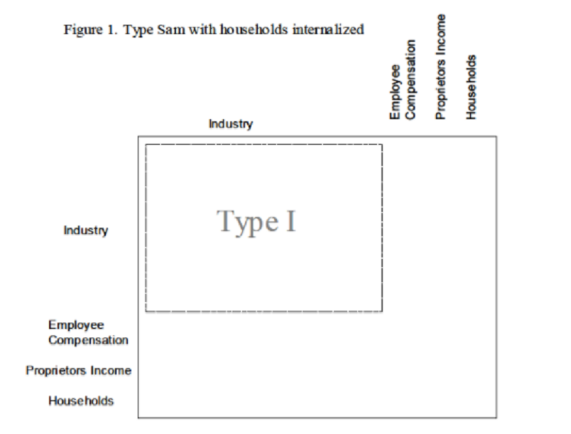
Type SAM Multipliers with Households Internalized
Theoretically, you could internalize any of the Institutions (households, government, and capital), but the standard practice (and the default in IMPLAN) is to internalize households only; that is, to capture the household spending of Labor Income but not the spending of tax revenues or returns to capital (Figure 1).
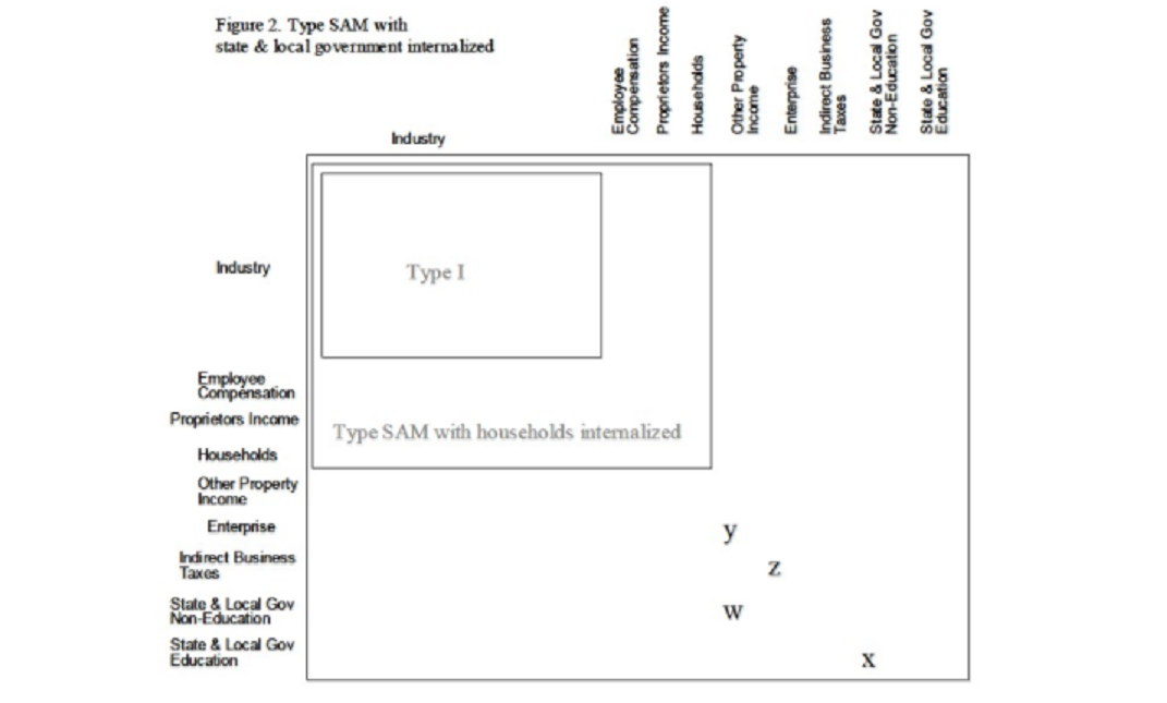
Type SAM Multipliers with State and Local Government Internalized
Internalizing State & Local Government Education and Non-education assumes that these Institutions will re-spend each dollar of local tax, fee, licenses, etc. collected locally for local programs. In a state model this makes sense – state budgets are required to be balanced, so the more they collect the more they spend and vice-versa (the occasional state tax rebate complicates this but it tends to be the exception rather than the norm). At the local level, however, this becomes more problematic; while the locally-collected tax dollar goes to the state general pot, the local region tends to receive equal money back (the occasional newspaper article pops up regarding a local legislator complaining that his district is not receiving its fair share of state revenue. Likewise, a declining region will receive more than its fair share of unemployment compensation and economic development funds).
Figure 2 helps illustrate the mechanics of internalizing State & Local Government. First note that we have introduced Other Property Income (OPI), which is mostly corporate profits, and Enterprises, which is mostly retained corporate profits. These have been included because for some states corporate taxes are an important source of government income. There is a direct transfer of interest (either net positive or negative) marked as “w” in Figure 2 from OPI to Government. There is also a transfer from OPI to Enterprises (the source of retained earnings) – marked “y” in Figure 1 and the transfer from Enterprises to State and Local Government Non-Education (corporate income taxes) – marked “z” in Figure 2.
Taxes on Production & Imports (sales taxes, property taxes, licenses, etc.) represent one of the most important sources of income for State and Local Government. Note that payroll taxes and personal income taxes are already part of the default formulation with households internalized. If including a State and Local Government Institution, it is almost necessary to include both Non-Education and Education together in the formulation because a large portion of State and Local Non-Education spending is an appropriation to Education. In IMPLAN, only the Non-Education Sector collects money, so Education is only funded by an appropriation. If internalized by itself, this would not add any impact to the Induced Effects. Thus, without Education, a large portion of the Non-Education spending would be leaked.
However, the case for State and Local Government Investment is not as straightforward. While much of Government Investment is operational capital goods (trucks, computers, etc.), very large projects (highways, buildings, stadiums, etc.) are funded through bonding and are not necessarily related to the current state of the economy. IMPLAN is not aware of any studies in which Government Investment is internalized as part of a Type SAM Multiplier.
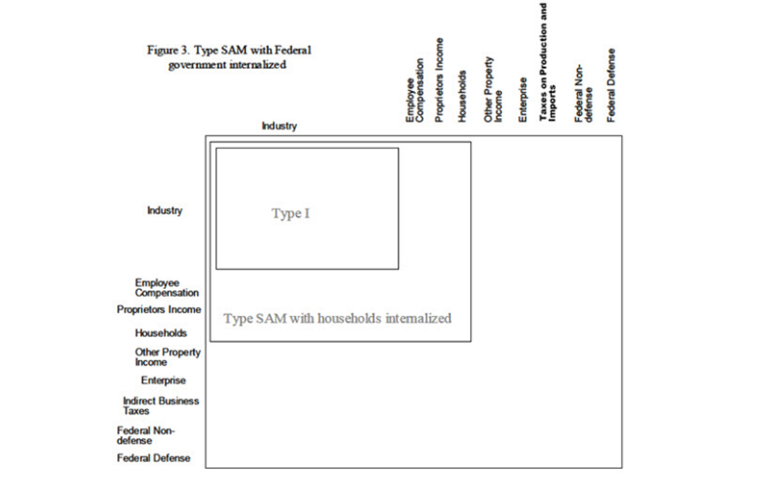
Type SAM Multipliers with Federal Government Internalized
Internalizing Federal Government is similar to internalizing State and Local Government in that it assumes that each dollar of locally-collected Federal taxes will be re-spent locally. The only situation where internalizing Federal Government can be safely justified is in a national Model. Many Federal Non-Military services are based on population and some argument could be made to include it, but the ability of more powerful representatives to direct appropriations render this assumption questionable at the local level. When it comes to Federal Military, a locally growing economy will cause little Indirect or Induced growth on the local military base, rendering this assumption questionable at the local level as well. The formulation of the type SAM Multiplier with Federal Government internalized (Figure 3) mirrors that with State and Local Government internalized. Federal Non-Military funding comes from taxes paid by Households, Taxes on Production & Imports (TOPI), corporate income taxes, and net interest payments from OPI. One increasingly significant source of Federal funding is Capital (i.e., borrowing). However, Federal borrowing is not linearly related to the economy, so it is not included as part of the type SAM Multiplier. Similar to State and Local Education (above), Federal Military is only funded by appropriation from Federal Non-Military, so by itself would not add to the Induced Effect.
Internalizing Federal Government Investment is even more tenuous than State and Local Government Investment. Federal Investment is likely to be more directly related to the party and seniority of the representative or the occurrence of a disaster than local economic conditions. Local economic factors figure very little in Federal spending decisions, except to the extent that population (i.e., voters) grow and decline. Since a Federal response to a new local factory is unlikely, we cannot recommend internalizing any Federal Institution.
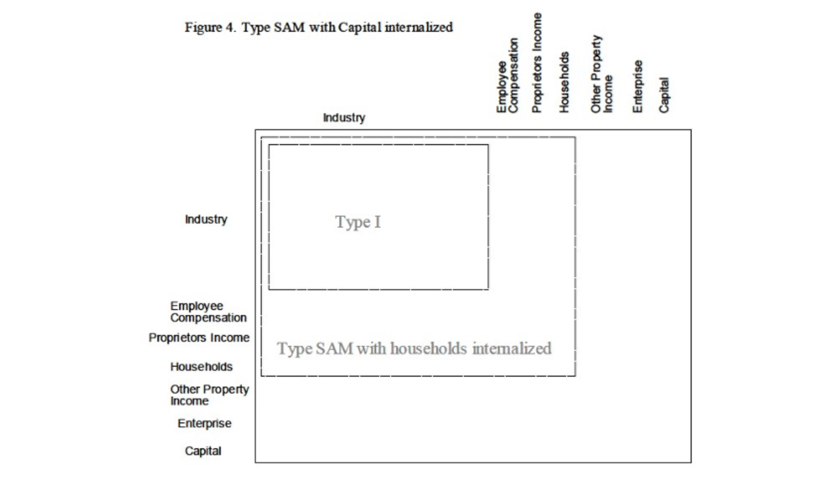
Type SAM Multipliers with Capital Internalized
Capital formation (purchase of new structures and capital equipment) is not part of any Industry production function. These purchases are a separate Institution forming one of the components of Final Demand. Final Demand is the final consumption of a good for the region – goods and services that are part of capital formation have met their ultimate use. Buildings and equipment are not re-manufactured creating new Value Added (however, they can be resold as used goods).
Industry decisions to invest are based on local conditions and perhaps the business cycle. If conditions are correct, they will invest (a non-linear action) with the promise of using a future stream of increased Value Added to pay off the investment. What this means is that when you cause an impact, increasing the Induced demand for restaurant Output (for example), we get the Employment, income and operational spending to run the restaurant but the Multipliers do not incorporate any economic activity associated with the construction of the restaurant.
Figure 4 shows the formulation of the Type SAM Multiplier with Capital Internalized. Sources of income for capital come from Industries (in the form of sales of scrap and used goods), from Households (in the form of sales of scrap and used goods and savings) and from Enterprises (in the form of savings from Other Property Income retained earnings).
As a region grows, you would expect investment to grow accordingly – but invetment is not based on local saving, but is a function of business cycle and how mature (how much of its infrastructure needs are in place) the region is. Also, this really could only possibly work in the growth direction. As a region declines, its savings decline, which would force the Multipliers to respond to negative investment.
The only rationale for negative investment is the curb on growth excess capacity has on regional investment when the region starts to grow again.
Type SAM Multipliers with Enterprises (Corporations) Internalized
There is no real spending pattern for retained earnings other than distribution to owners, government, and savings. As such, it may be useful to internalize Capital together with those Institutions but not on its own. At the local level, owners are quite likely to live outside of the region, which is why it is not standard practice to internalize this Institution.
Type SAM Multipliers with Inventory Internalized
Changes in inventory levels allow for calculating Gross Regional Product and for balancing production with sales but have no real economic impact interpretation if internalized.
https://implan.com/wp-content/uploads/Market-site-Logo-resized-2-1.jpg00Adam Smithhttps://implan.com/wp-content/uploads/Market-site-Logo-resized-2-1.jpgAdam Smith2019-10-24 16:42:322019-10-24 16:42:44Explaining the Type SAM Multiplier
Wassily Leontief is referred to as the “father” of I-O analysis, for which he received the Nobel Prize in 1973. Beginning in the 1930s, he constructed the first I-O tables for the United States, and he also served as a consultant to the Bureau of Labor Statistics when they published the first official U.S. I-O table in 1944. (BEA)
Generated by the model building process, the Social Account Reports Table and the Balance Sheets Table both contain a wealth of information about the specified study region. Provided below are definitions and descriptions of many of the terms and categories found within the two tables.
Social Account Reports Table
Commodity Summary
Industry Commodity Production = the total output of this commodity that is produced by industries. Some commodities are produced by more than one industry – this value includes the sum of the production of this commodity by all industries.
Institutional Commodity Production = the total output of this commodity that is produced by institutions (i.e., produced by Government or taken out of Inventory).
Total Commodity Supply = Industry Commodity Production + Institutional Commodity Production.
Net Commodity Supply = Total Commodity Supply – Foreign Exports of the commodity from the region. Foreign Exports can be found by selecting View By: Commodity Trade.
Intermediate Commodity Demand = total demand for this commodity by industries.
Institutional Commodity Demand = total demand for this commodity by institutions (Inventory, Government, Households, Capital).
Total Gross Commodity Demand = Intermediate Commodity Demand + Institutional Commodity Demand. The term “gross” refers to the fact that these figures include imports (both foreign and domestic) of the commodity into the region.
Domestic Supply/Demand Ratio = the percentage of total local demand for the commodity that could possibly be met by local production. It is calculated by dividing Net Commodity Supply by Total Gross Commodity Demand, constrained to a maximum of 100%.
Average RPC = the proportion of local demand for the commodity that is currently met by local production. It is “average” in the sense that there is just one RPC per commodity, so all industries and institutions are assumed to purchase that commodity locally at the same rate.
Average RSC = the proportion of local supply of the commodity that goes to meet local demand.
Commodity Trade
Foreign Exports = output value of local production of this commodity that is exported abroad.
Domestic Exports = output value of local production of this commodity that is exported to other regions of the U.S.
Total Exports = Foreign Exports + Domestic Exports
Intermediate Imports = value of imports (both foreign and domestic) into the region for use by industries as an input.
Institutional Imports = value of imports (both foreign and domestic) into the region for final use by institutions (Inventory, Government, Households, Capital).
Total Imports = Intermediate Imports + Institutional Imports.
Foreign Export Proportion = the percentage of Total Exports that go to foreign countries. It is calculated by dividing Foreign Exports by Total Exports.
Institution Local Commodity Demand
This table lists each institution’s demand for local production of each commodity. The sum across all institutions for a particular commodity is the total local institutional demand for local production of that commodity. This sum is equivalent to Institutional Commodity Demand * Average RPC from the View By: Commodity Summary screen. Foreign Exports and Domestic Exports are the same as reported in the View By: Commodity Trade screen.
Household Local Commodity Demand
This table lists each Household type’s demand for local production of each commodity. The sum across all Household types for a particular commodity is equivalent to the “Households” value in the View By: Institution Local Commodity Demand screen.
Government Local Commodity Demand
This table lists each Government type’s demand for local production of each commodity. The sum across all Government types for a particular commodity is equivalent to the “Government” value in the View By: Institution Local Commodity Demand screen.
Balance Sheets Table
Industry Balance Sheet
Commodity Production
Commodity Production = the output value of each of the commodities produced by this industry.
Market Share = the proportion of Commodity Production that is produced by this industry. If there is more than one producer of a commodity, this industry’s Market Share for that commodity will be less than 100%.
Byproduct Coefficient = the proportion of this industry’s total industry output that is dedicated to each commodity. If the industry makes more than one commodity, each Byproduct Coefficient will be less than 100%.
Commodity Demand
Gross Absorption = the proportion of Total Industry Output for this industry that goes toward purchases of each commodity. Gross Absorption is calculated as Gross Inputs/Total Industry Output. Total Gross Absorptions will be less than one, with the remainder of Total Industry Output going toward Value-Added.
Gross Inputs = the value that this industry spends on each commodity.
RPC = the proportion of local demand for the commodity that is currently met by local production. This is the same value as that found in the View By: Commodity Summary screen.
Regional Absorption = the proportion of Total Industry Output for this industry that goes toward local purchases of each commodity. Regional Absorption can be calculated as Gross Absorption * RPC.
Regional Inputs = the value that this industry spends locally on each commodity. Regional Inputs can be calculated as Gross Inputs * RPC.
Value Added
Value Added Coefficient = the proportion of Total Industry Output that goes toward each category of Value-Added. Each Value Added Coefficient can be calculated by dividing Value Added by Total Industry Output. The Total Value-Added Coefficient + Total Gross Absorption = 1.00.
Value Added = the dollar value paid to each category of Value Added.
Commodity Balance Sheet
Industry-Institutional Production
Industry Production = the total output of this commodity that is produced by the industry listed in each row.
Market Share = the proportion of Industry Production that is produced by the industry/institution listed in each row. If there is more than one producer of this commodity, each Market Share will be less than 100%.
Byproduct Coefficient = the proportion of each industry’s total industry output that is dedicated to this commodity. If the industry/institution makes more than one commodity, the Byproduct Coefficient will be less than 100%.
Industry Demand
Gross Absorption = the proportion of Total Industry Output for each industry that goes toward purchases of this commodity. Gross Absorption is calculated as Gross Inputs/Total Industry Output.
Gross Inputs = the value that each industry spends on this commodity.
RPC = the proportion of local demand for the commodity that is currently met by local production. This is the same value as that found in the View By: Commodity Summary screen.
Regional Absorption = the proportion of Total Industry Output for each industry that goes toward local purchases of this commodity. Regional Absorption can be calculated as Gross Absorption * RPC.
Regional Inputs = the value that each industry spends locally on this commodity. Regional Inputs can be calculated as Gross Inputs * RPC.
Institutional Demand
Gross Demand = the amount that each institution spends on this commodity.
RPC = the proportion of local demand for the commodity that is currently met by local production. This is the same value as that found in the View By: Commodity Summary screen. Note that if institutions purchase this commodity from local retailers, the retail margin portion of the purchase will have a high RPC; however, the producer portion of the purchase price will have a low RPC if there is little local production of that commodity.
Regional Demand = the amount that each institution spends locally on this commodity. Note that this value has already been margined (that is, if the institution buys this commodity from a retailer, this value only shows the portion of that purchase amount that goes to local producers of the commodity). Regional Demand can be calculated as Gross Demand * RPC.
https://implan.com/wp-content/uploads/Market-site-Logo-resized-2-1.jpg00Adam Smithhttps://implan.com/wp-content/uploads/Market-site-Logo-resized-2-1.jpgAdam Smith2019-10-24 16:40:522019-10-24 16:41:52Understanding the Social Accounts Tables
Method of valuing inventories that assumes that the most recent addition to inventories is sold first. (BEA)
https://implan.com/wp-content/uploads/Market-site-Logo-resized-2-1.jpg00Joe Demskihttps://implan.com/wp-content/uploads/Market-site-Logo-resized-2-1.jpgJoe Demski2019-10-24 16:40:062019-10-24 16:40:33Last in, first out (LIFO)
The full-detail Social Accounting Matrix (SAM) gives a complete picture of the flow of funds, both market and non-market, throughout the economy in a given year. Market flows occur between the producers of goods and services (both industrial and institutional) and the purchasers of those goods and services, both industrial and institutional (i.e., households, government, investment, and trade). Non-market flows occur between institutions (e.g., between households and government, between households and capital, etc.) and are often called inter-institutional transfers. In such transactions there is no well-defined market value being exchanged in return for the payment; for example, while taxes are used to fund government services, these government services do not have a market value since they are not purchased in a market setting. In a typical SAM, the columns represent payments or expenditures by the column industry, commodity, or institution, while the rows represent a receipt of income by the industry, commodity, or institution.
National SAM
The U.S. SAM data come directly from the BEA’s National Income and Product Accounts (NIPA) data, with the exception of the institutional trade and capital accounts, which are calculated as part of the balancing routine. Balancing refers to the act of forcing each row sum to equal its corresponding column sum; balancing is necessary due to varying levels of precision and resulting rounding discrepancies in the data used to construct the SAM.
Sub-National SAM Data
With the exception of some inter-institutional transfers, the majority of the state, county, and zip code SAM data come directly from the regional IMPLAN industry data estimated as described here. The software allocates the remaining national SAM data to states, counties, and zip codes based on our IMPLAN industry data and other regional data. The software then combines these data with the industry data and balances the institutional trade and capital accounts to form a balanced regional SAM.
Household Transfers
Estimates of household income and transfer payments come from several sources, including the following:
IMPLAN industry data (estimated as described here)
REA tables CA35 (personal current transfer receipts) and SA50 (personal current taxes)
NIPA Personal Consumption Expenditures (PCE)
BLS Consumer Expenditure Survey (CES)
The Annual Survey of State and Local Government Finances
The Census Bureau’s State Government Tax Collections series
The Census Bureau’s Journey-To-Work data
Labor income received from industries is provided by IMPLAN industry data and is place-of-work income. Household income data, by contrast, are place-of-residence. The REA data include a residency adjustment, as well as some transfer payments data.
Household personal consumption expenditures are derived from the NIPA PCE data, with household income category detail obtained from the CES data. The national data are distributed to states and counties on the basis of the area’s total household spending in each household income category. It is assumed that within a given income group, taxation and spending patterns are similar across the nation. While the CES data are available for 6 regions, analysis by IMPLAN did not show statistically significant differences in expenditure patterns across regions for a given household income category.
Taxes are regionalized to states and counties based on tax collection totals from the Annual Survey of Government Finances and the Census Bureau’s State Government Tax Collections series.
Government Transfers
The BEA NIPA datasets provide the control totals for government transfers. These control totals are allocated to states and counties based on IMPLAN industry data as well as data from the Annual Survey of State and Local Government Finances and the Census Bureau’s annual State Government Tax Collections series.
Enterprise
Enterprise is distributed based on estimated output for the region.
Capital
Payments by capital to other institutions represent net borrowing of money by that institution. Payments by other institutions to capital represent net savings by that institution. The capital accounts are a balancing item that is allowed to float. If the other elements are specified correctly, the capital accounts will be accurate.
Inventory
Inventory change is distributed based on estimated output for the region.
Trade
Payments by trade to other institutions represent a flow of money into the region from outside. Payments by other institutions to trade represent a flow of money from the region to other regions. Domestic imports and exports of commodities are specified as described here. Trade flows of labor income (i.e., commuter flows) are captured by Census Journey-To-Work data. The remainder of the trade entries are used for balancing.
Please see this article for more details on the structure of the IMPLAN SAM.
https://implan.com/wp-content/uploads/Market-site-Logo-resized-2-1.jpg00Adam Smithhttps://implan.com/wp-content/uploads/Market-site-Logo-resized-2-1.jpgAdam Smith2019-10-24 16:39:312019-10-24 16:39:51SAM Data Development
Labor Income Events are most appropriate to use when an analyst intends to model a change in labor payments isolated from an industry’s production. When creating a Labor Income Event in IMPLAN, analysts may specify whether the income is earned by wage and salary employees, by sole proprietors, or some combination of the two. However, they cannot specify the specific household income categories which will receive that income.
https://implan.com/wp-content/uploads/Market-site-Logo-resized-2-1.jpg00Joe Demskihttps://implan.com/wp-content/uploads/Market-site-Logo-resized-2-1.jpgJoe Demski2019-10-24 16:38:542019-10-24 16:39:06Labor Income Events