The Curious Case of the Negative Tax: Agriculture Subsidies, Profit Losses, and Government Assistance Programs

INTRODUCTION:

One of the most frequent questions we get at IMPLAN is “Why am I seeing negative taxes in my impact?”  Good news, there are reasons that this happens. This article breaks down how to find those negative figures and why they are there. 

AGRICULTURE SECTORS:

The agriculture Sectors in IMPLAN see significant amounts of government subsidies.  Agriculture subsidies are payments by the federal government to farmers “for the purpose of stabilizing food prices, ensuring plentiful food production, guaranteeing farmers’ basic incomes, and generally strengthening the agricultural segment of the national economy” (Encyclopedia.com).

Taxes on Production & Imports less Subsidies (TOPI) is one of the four components of Value Added.  All payments to government, other than payroll/personal taxes and year-end corporate income taxes, are paid through TOPI. TOPI varies a lot year to year because of how agriculture products Commodity prices vary, weather, and global market shifts.  

In general, negative TOPI is due to the given Industry receiving subsidies from the government. As TOPI is typically tax payments to the government, it follows that a negative TOPI value suggests a receipt of money from the government. Because TOPI is net of subsidies, it can be negative for a given Industry in a given year, if that industry received more subsidies from the government than it paid out in these specific taxes in that year.  

curious_case_1.jpg

The TOPI by IMPLAN Sector can be examined on the Regions screen by navigating to Region Details > Study Area Data > Industry Detail.

In Illinois, for example, we see that Sector 1 – Oilseed farming had a TOPI of negative $2,760,684.85 in 2017.  In fact, all of the first five agriculture Sectors had negative TOPI in Illinois that year.

IMPLAN uses data from the Bureau of Economic Analysis (BEA) by state.  Under Annual Gross Domestic Product By State, you can find tables for TOPI, TOPI less subsidies, and subsidies. Beginning in in Data Year 2015, IMPLAN incorporated USDA ERS Agriculture Resource Management Survey (ARMS) data to estimate components of value added by commodity at the national and state levels.  ARMS reports government payments, ie, subsidies, real estate and other property taxes (a large component of gross TOPI for farm sectors), interest (a component of OPI), and depreciation (another component of OPI). For details on the methodology, visit our article on Farm Data Procedures.

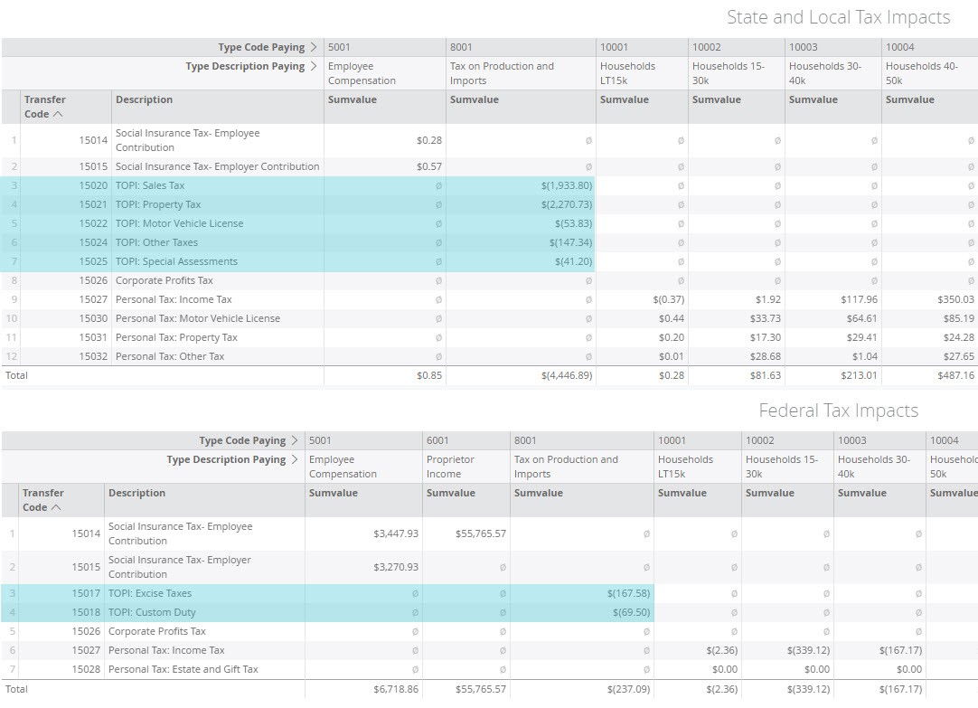
Staying in the Prairie State, let’s say we want to see the impact of $10M in sunflower production, Sector 1 – Oilseeds.  On our Results screen, we filter for the Direct Effect to see negative TOPI at the State & Local and Federal levels.

curious_case_2.jpg

Note that the split across the different TOPI line items is regionally specific.  However, there are no Industry-specific breakouts of TOPI: the negatives in one part (i.e. subsidies) gets shared out to all parts of TOPI (i.e. sales tax, property tax, etc.).  

OTHER SECTORS:

Agriculture Sectors are not the only places that we can see negative taxes. Additionally, TOPI is not the only component of Output from which negative taxes stem from.  Usually, businesses make money and therefore we see positive profits. However, this isn’t always the case. As Other Property Income (OPI) is mostly made up of corporate profits, this is also were we will see corporate losses.

Modeling a $10M stock broker firm in Illinois (Sector 435 – Securities and commodity contracts intermediation and brokerage), illustrates this example.  Again, filtering for our Direct Effect on the Tax Results tab, we see negative results in Private Enterprises payment to Corporate Profits Tax, which is stemming from a payment from OPI.

curious_case_3.jpg

In detail, these losses to an Industry would be reflected by negative Other Property Income (OPI) or by negative Proprietor Income (PI) if the loss is to a self-employed owner. OPI and PI by Sector can also be viewed in Region Details > Study Area Data > Industry Detail.

Heading to the Value Added tab on the Results screen, we can drill down into the details on EC, PI, TOPI, and OPI.  Sorting by the totals for PI, we see that the $10M investment in the stock broker firm has an associated negative PI of $173,768.13.  This demonstrates that overall in Illinois in 2017, proprietors in this Sector lost money.

curious_case_4.jpg

Scrolling further down the Value Added details page, we can sort the OPI table to see that the $10M stock brokerage has an associated negative $2,154,647.86 in OPI.  

curious_case_5.jpg

HOUSEHOLDS:

The other place you will see negative taxes is actually in households.  Running $10M through for a fast food restaurant (Sector 502 – Limited-service restaurants) illustrates this point.  

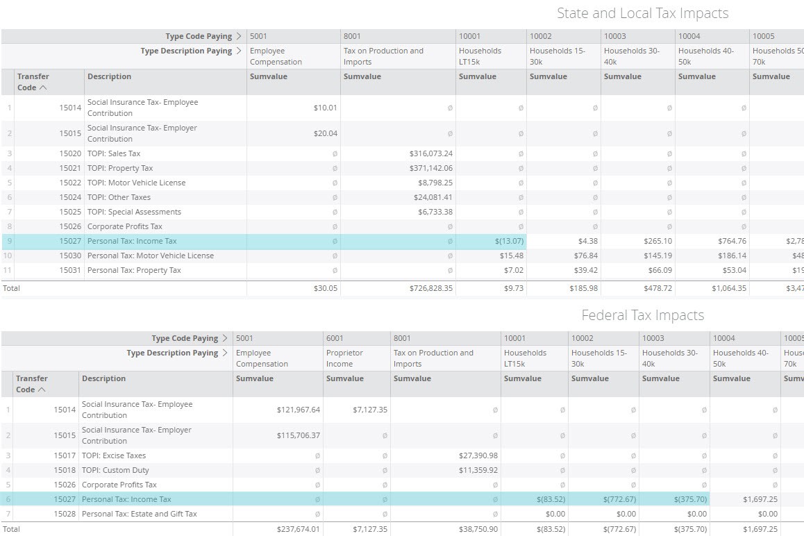
At the State and Local level, Households earning less than $15k/year see negative $13.07 in personal income tax from the $10M impact.  This means that households in this bracket are seeing a refund from the government or are receiving more in benefits (like food or housing) than they pay in taxes.

At the Federal level, three income groups see negative values for personal income tax.  This again represents tax refunds that these households see or that the amount of benefits they receive outweighs the amount of taxes they pay.  

The portion of personal taxes paid by Households for each dollar they earn are income group and Region specific, but not sector specific. Similarly the portion of payroll taxes paid out of Employee Compensation and Proprietor Income for each dollar earned are specific only to the Region, not the industry. 

curious_case_6.jpg

RELATED ARTICLES:

Farm Data Procedures

Generation and Interpretation of IMPLAN’s Tax Impact Report

Non-comparable imports

NEC

NAPCS

Economic Impact, Economic Contribution, and Export Base

Introduction

The purpose of this paper is to clarify the differences between three commonly confused terms and methods in the more general realm of input-output (I-O) analysis: economic impact analysis, economic contribution analysis, and gross-base analysis.  While each of the three types of analyses has a distinct purpose and method, they all rely on data from an I-O model, which itself is a bit of a misnomer.  When first popularized by Wassily Leontief, I-O tables focused on the purchasing behavior (input) and production (output) of industries only.  Later, the purchasing, producing, saving, and investing behavior of institutions such as governments and households was also added to the I-O tables, forming what is now known as a Social Accounting Matrix (SAM) and spurring a corresponding name change from I-O models to SAM models.

Please note that in the discussion that follows, Output is used as the measure of interest, though the same principles apply to Employment and any of the individual components of Output.  Please also note that we have included a technical section that gives a detailed numerical demonstration of IMPLAN’s recommended contribution analysis methods and their relationship to the established literature.


Economic Impact Analysis

In a typical final demand change (i.e., “impact”) analysis, the analyst is modeling a new firm or a change in the level of Output of a given firm.  In such cases, the Direct Effect is the new firm’s total Output or the existing firm’s change in Output.  In such cases, it is likely (and logical) that the industry in which that firm belongs will experience total impacts that exceed the direct impacts – that is, the industry will experience indirect and induced effects that stem from the direct effects. 


Consider the example of wood window and door manufacturing in Washington County, MN.  This industry already exists in the county, with Anderson Windows being one of the existing firms in this industry in Washington County.  Now suppose a new wood windows and doors manufacturer, Wonder Windows, is planning to locate in Washington County with expected Output of $5 million dollars.   This new plant would create new demand for some local businesses (the purchase of dimension lumber and preserved wood products, for example), which may spur some of these local businesses to undertake building improvements or expansions, thereby necessitating new windows, thereby creating indirect demand for the wood windows and doors sector.  Additionally, most firms make purchases from other firms in their own industry (for example, consulting services, equipment rental), which generates additional indirect demand for that same industry.  In addition to these indirect effects, the new Wonder Windows plant would also attract some new workers to the region, spurring home improvements to some existing homes and apartments, thereby generating induced demand for the wood windows and doors industry.  Such “feedback” effects to the industry are part of that industry’s overall impact in the region.

Contribution Analysis – Extraction Method

However, there are occasions when an analyst would like to see the indirect and induced effects that the current level of Output of an existing industry as a whole has on other industries in that region.  In this case, the goal is to generate a total Output effect on the primary industry of interest that is equal to the current level of production of that industry, while showing the indirect and induced effects that this current level of Output has on other industries in the region.  In other words, the only “effects” that the industry of interest should experience are the direct effects (e.g., current Output), while other industries in the region experience indirect and induced effects associated with (i.e., in support of) the direct effects in the industry under study.  In such a study, it does not make sense to allow feedback effects on the primary industry of interest, since an existing Industry cannot experience a total Output “effect” that exceeds its current level of Output.  In other words, the question of contribution analysis assumes by definition that the effect on the sector whose contribution is being measured is the entire value of its own Output.[1]

As another example, consider the shutting down of an industry.   If the current level of industry Output were to be modeled as a negative direct effect using the traditional impact analysis approach, the model would show a total loss to this industry that is greater than its current level of Output – but it’s not possible to lose more Output (or Employment) than currently exists! 

Therefore, special modeling techniques are required in these cases to ensure that the results accurately reflect the addition/loss of just the projected/current level of Output of the industry of interest plus the indirect and induced effects in other industries.  This is the purpose of what we at IMPLAN term Contribution Analysis.  The basic idea is to disallow indirect or induced purchases from the industry of interest in such a way that does not affect the indirect and induced effects on other industries.  In the input-output literature, these methods often are called “mixed endogenous-exogenous models.” 

If the industry of interest produces just one type of commodity (e.g., wood windows and doors), this is accomplished by setting the regional purchase coefficient (RPC)[2] for that commodity to zero.  If, on the other hand, the industry of interest produces additional commodities as by-products of the production of its primary commodity (e.g., cut stock, re-sawn and planed lumber), it is necessary to either a) modify the model to assume that the industry only produces its primary product or b) set the RPC for each of the industry’s by-products to zero.  This method can be used for both single- and multi-industry contribution analyses, and instructions to do so in IMPLAN can be found on the IMPLAN website, currently at https://implanhelp.zendesk.com/hc/en-us/articles/115009542247-Multi-Industry-Contribution-Analysis-In-IMPLAN-Pro.  This is a similar approach to that described in Miller and Blair’s seminal input-output modeling textbook (2009, pp. 624-625 and Appendix 13.2), although they zero out local purchases from the primary industry directly in the A matrix, whereas in IMPLAN we zero them out indirectly by way of multiplying them by an RPC of zero. 

When performing a contribution analysis on a single industry, an alternative approach, also recommended by Miller and Blair, is available.  It involves starting the analysis with a direct Output effect reduced by a factor of that industry’s detailed multiplier on itself, accomplished by dividing the industry’s current Output by its detailed output multiplier on that same industry.  When this approach is used, there are indirect and induced Output impacts on the original industry that, when summed with the appropriately reduced direct Output, reproduce the original (i.e., current) level of total Output in that industry, and thereby also generate the appropriate indirect and induced effects in other industries, equal to those generated by the RPC method above.  The only difference between the results is that with this method, the “indirect” and “induced” effects on the primary industry must be reclassified as “direct” effects.  A limitation of this approach is that it can be used only when analyzing a single industry, but an advantage of this approach is that the industry in question is allowed to produce more than one commodity (i.e., no need to reduce the number of by-products to just the one primary commodity).  This approach is described in Miller and Blair (2009, p. 625).  Instructions for performing this type of analysis in IMPLAN can be found on the IMPLAN website, currently at

https://implanhelp.zendesk.com/hc/en-us/articles/115002812694-Estimate-the-Contribution-of-a-Single-Industry-in-IMPLAN-Pro [3]

A criticism of the multi-industry contribution analysis methodology is that, if one were to perform the analysis for all industries simultaneously, the only “impacts” would be the direct impacts (i.e., the gross outputs of every industry), with no indirect or induced impacts.  In other words, there would be no new information gained from such an exercise.  We agree that there indeed is no point to such an exercise, since it assumes its own conclusion; but, that neither invalidates the approach nor negates its usefulness when used to examine any number of sectors less than all possible sectors.

In the technical section of this paper, we present a numerical analysis that explains IMPLAN’s contribution analysis methods in reference to established input-output literature and demonstrates their consistency and appropriateness for the contribution analysis problem.


Contribution Analysis – Gross-Base Method

In gross-base contribution analysis, the goal is not to determine what would happen were a sector to disappear from the local economy, but rather to determine the output (or employment, etc.) required by all local industries in support of that region’s exogenous demands, which consist of demands by all non-internalized institutions.[4]  We argue that gross-base contribution analysis is a straightforward variant of impact analysis, not a substitute for extraction-based contribution analysis.  The context of the analysis determines the preferable method.

Gross-base contribution analysis, as described in Watson et al. (2015), makes one noteworthy deviation from typical impact analysis.  It tabulates exogenous demands as a diagonal matrix rather than as a column vector, which gives a matrix of resulting output, rather than a column vector of gross output.  It uses the same multiplier matrix as traditional impact analysis; again, the only difference is the dimensionality of the exogenous demand vector.  If one models exogenous demand only for a single industry, gross-base analysis is indistinguishable from impact analysis, since both results will be column vectors of identical value.

In gross-base analysis, internalization considerations (also known in the literature as the model closure) are the same as they are for impact and extraction analysis.  Internalizing affects assumptions about re-spending in the local economy: at the county level, for example, internalizing federal government implies that federal spending in a particular county is a linear function of federal tax revenue collected due to economic activity in the county.  For more information on internalizing institutions, please see this article: http://support.implan.com/index.php?view=document&alias=56-type-sam-multiplier&category_slug=studies-1&layout=default&option=com_docman&Itemid=1764.

Additionally, note that the gross-base method is not a mixed exogenous-endogenous model.  For any given institution, it treats either all or none of that institution’s demand as exogenous, rather than extracting certain industries, e.g., agriculture, by characterizing agriculture as exogenous and the remaining industries as endogenous.  The methods recommended by Miller and Blair for “extracting” a sector involve treating some industries as exogenous and the rest as endogenous, and recalculating the multiplier matrix (the Leontief inverse) after adjusting for these specifications.  The practice of multiplying exogenous demand, when defined for all institutions of a particular type, regardless of whether that demand is all final demand, only some of final demand, or only exports, by its corresponding multiplier matrix better resembles impact analysis than it resembles extraction contribution analysis.

Using either a diagonal matrix or a column vector of exogenous demands performs the same mathematical operation.  The only difference is that using the diagonal matrix effectively pauses the calculation before summing each row in the result set.  The sum of the elements in a row of the product of a multiplier matrix and consistently defined diagonal matrix of final demands yields the same values that would result were a column vector of exogenous demand to be used; moreover, the column vector approach gives each element that the diagonal exogenous approach yields as one of the steps in its calculation.  Simply put, if one used the column vector approach and stopped before finishing it, the values would be the same as what the diagonal matrix approach gives.  The individual elements of the sum, however, are informative in their own right and, depending on the context, may be worth reporting and analyzing.  Watson et al. characterize the sum of the columns, rather than of the rows, as “base” output.

Accordingly, we believe that the methodology outlined in Watson et al. (2015) would be better termed base-gross contribution analysis and that it should not be confused with extraction contribution analysis, since it is incapable of consistently estimating the effect of extracting an entire sector.[5]  Using the multiplier matrix recommended in Watson et al., and applying an industry’s total output as the direct effect would result in an output effect larger than the total output.  Similarly, using only final demand for a single industry as the direct effect would not reproduce all of that industry’s gross output, some of which goes to support intermediate production in other industries.  In other words, it is ill-suited to answering the question of what would happen if an industry were to disappear in an input-output framework.  It appears well-suited, however, to performing “base analysis” for a given specification of a model’s closure (i.e., its specification as to which institutions are internalized/endogenous).  Classifying exports as the only exogenous demand is the approach often adopted in gross-base analysis, and has sometimes been termed “export base analysis.”  The method of using a diagonal vector of exogenous demands, however, can be applied to any model closure (internalization) specification.  To recover total industry output for all industries, however, the exogenous demand vector needs to include all institutions not internalized in the model.  Overall, studying the components of the product of the multiplier matrix and diagonalized matrix of exports (or other combination of demand elements that have been classified as exogenous) can be informative in its own right, as explained by Watson et al., but ought to be classified as a distinct method.  In short, base output for a given sector represents the effect of modeled exogenous demand for the given sector on all other sectors; gross output for a given sector, in turn, represents the effect of modeled exogenous demand for all other sectors on the given sector.


Technical Section: Internal Consistency of IMPLAN’s Contribution Analysis Methods

In this section, we demonstrate via numerical examples that IMPLAN’s two methods for extraction contribution analysis – single industry and multi-industry – are internally consistent with the model, consistent with the existing literature, and consistent with each other (that is, the multi-industry approach, when used for a single industry, will replicate the results of the single-industry approach).

To establish a common terminology and notation, we briefly review the basic input-output (I-O) model.  The common specification of a basic I-O model holds that intermediate inputs plus final demands equals gross output.  Algebraically, in matrix form, let A be a be a matrix of intermediate input ratios, I be the identity matrix, y be a column vector of final demand by sector, and x be a column vector of gross output by sector.  The y vector also can be described more generally as “exogenous demand.”  In the basic I-O model specification, all of final demand – that is, household demand, government demand, investment demand, net inventory additions, and export demand – is classified as exogenous.  What the modeler chooses to classify as exogenous is implied by what is internalized in the model.  If only industries are internalized, all of final demand is exogenous (this is the specification for IMPLAN’s Type 1 multipliers).  If industries and households are internalized (the default specification for IMPLAN’s Type SAM multipliers), then only demand by governments, capital investment, inventory, and exports are exogenous.  Another way to think of this is that payments to institutions that are considered exogenous are “leaked” from the economy, whereas some portion of payments to endogenous institutions (usually industries and households in IMPLAN) are re-spent locally.  According to the Leontief equation, x = Ax + y.  Rearranging, xAx = y, and, factoring out x, (IA)x  = y.  The matrix of multipliers is found by identifying the matrix by which exogenous demand can be multiplied to reach total output, which is the inverse of (IA).  Put differently, for a given amount of exogenous demand, multipliers tell how much total output needs to be produced by each industry.  One multiplies the inverse of (IA) by both sides of the equation to reach the solved equation, which is (IA)-1y = x.  This definition provides a test of the consistency of an input-output model.  If any two of the three elements (multipliers, exogenous demands, and gross outputs) can be used to find the previously-known third element, then the model should be considered internally consistent.

For the numerical illustrations below, we use 2014 IMPLAN data for the United States, aggregated to 5 sectors and a single household type.  We begin with a basic I-O model, not yet attempting to perform a contribution analysis.  Figure 1 shows the IxI SAM, with exogenous demands (final demands, in this case) highlighted in green, endogenous spending highlighted in yellow, leakages in orange, and transfers in light yellow.  Exogenous demands are summed by row in the rightmost column.  Figure 2 shows the corresponding multiplier matrix, which is based on an A matrix from just the endogenous industries and institutions (only the industries in this case), also shows sums of exogenous demand, and multiplies the exogenous demands by the multiplier matrix.  The resulting vector is of gross output, which matches the initial gross output estimate.  Accordingly, the model is internally consistent when set up as a basic IO model in which all of final demand is exogenous and the multipliers are calculated according to the “Type 1” specification.

Figures 3 and 4 provide a corresponding setup based on the default IMPLAN Type SAM specification.  Figure 3 shows which components of the IxI are exogenous demands – now households are no longer exogenous – and which are endogenous.  The default Type SAM specification (or “model closure”) assumes that labor income payments are re-spent in the economy, less leakages to in-commuting and taxes.  Figure 4 shows that the Type SAM specification is internally consistent when the corresponding multiplier matrix is estimated and applied to the new set of exogenous demands.[6]

Next, we extend the Type SAM specification to demonstrate two different methods of contribution analysis.  As noted above, contribution analysis asks and answers the question of what would be the effects on all sectors’ output if an entire other sector (or sectors) were to disappear.  Miller and Blair describe this as “extracting” a sector and mathematically portray that by reclassifying the contribution sector(s)’ gross output as exogenous.  A necessary, but not sufficient, condition for a contribution analysis method to be consistent is that the method’s result must show that the entire gross output of the contribution sector(s) is lost.  That is, the result must reproduce the contribution sector(s)’s gross output.  Usually, another matter of primary importance in contribution analysis is the effect on all of the other sectors.  It follows that the other condition for a contribution analysis to be consistent is that the appropriate levels of multiplier effects on the non-contribution sectors are consistently estimated.  As noted above, an IO model can be deemed consistent if a set of exogenous demands and multiplier matrix reproduce gross outputs.

In the first example of contribution analysis, shown in Figures 5 and 6, the entire total output of sector 1 is exogenous, and the remaining sectors have their previous (i.e., default Type SAM-based) levels of exogenous demand.  Miller and Blair explain that a viable method for estimating any number of sectors’ contribution to the economy is to “zero-out” certain rows of the A matrix before calculating the multiplier matrix (p. 624-625, with general proof on p. 662).  IMPLAN’s method of zeroing-out RPCs achieves the same effect, as zero multiplied by the gross absorption rate for all industries equals zero, leaving zeroes in the A matrix for the contribution industry’s row.[7]  Figure 5 identifies exogenous and endogenous demands, and Figure 6 demonstrates that the new exogenous specification (all output of sector 1, as well as previously exogenous demands for the other sectors) reproduces gross output.  One can see that sector 1’s gross output is used as its exogenous (or “direct impact”) value, and is the same as the resulting value.

Note that Figures 5 and 6 merely show that this contribution analysis method is consistent.  Figure 7 then shows the results for one sector without including exogenous demands for the non-contribution sectors, as one usually is interested in just that one sector’s contribution to all other sectors’ output.  Figure 8 shows that the single-industry method, when used only on one industry, produces results identical to the multi-industry method as in Figure 7.  Recall that the single-industry method involves either dividing the leftmost column of the multiplier matrix by the own-sector multiplier (as in Miller and Blair, p. 625, with extensions following) or the algebraically equivalent function of dividing the top row of the exogenous demand vector by that same own-sector multiplier (as recommended by IMPLAN).

Since Figures 5 and 6 demonstrate the consistency of the multi-industry contribution analysis method, and Figures 7 and 8 confirm that the multi-industry method is consistent with the single-industry method when estimating the contribution of just one industry, it remains to be shown only that the multi-industry method is indeed consistent for more than one industry.  Figure 9 shows the identification of exogenous and endogenous payments.  Figure 10 demonstrates consistency: by specifying the gross output of the first two sectors as exogenous and using the ordinary exogenous demand for the remaining sectors, it reproduces gross output when multiplied by a multiplier matrix based on an A matrix with the first two rows zeroed-out.  Again, we rely on Miller and Blair for the formal mathematical demonstration that the method continues to be consistent for any number of “extracted”, or “contribution”, sectors.

Click here to find figures in the Word doc version of this article. 

Other Related Articles:

https://implanhelp.zendesk.com/hc/en-us/articles/115002801513-Considerations-of-Contribution-Analysis

References

Miller, R.E. and P.D. Blair. 2009. Input-Output Analysis: Foundations and Extensions, Second Edition.  New York: Cambridge University Press.

Watson, P., S. Cooke, D. Kay, and G. Alward. 2015. A Method for Improving Economic Contribution Studies for Regional Analysis. Journal of Regional Policy and Analysis, 45(1): 1-15.


[1] Economic contribution analysis usually is not, as stated in Watson et al. (2015), “generally regarded as referring to the ex post effects on economic activity in a region from the exogenous sales of a given sector in a previous time period.”  That definition typically applies to economic impact analysis.

[2] The RPC represents the proportion of local demand for a commodity that is met by local producers of that commodity.

[3] Miller and Blair’s example divides the first column of the multiplier matrix by the detailed multiplier, which is algebraically equal to, but computationally less efficient than IMPLAN’s recommended method of dividing the first row of the exogenous demand vector (i.e., the direct impact vector) by the detailed own-sector output multiplier.

[4] Exogenous demand is defined as demand by institutions that are not internalized in the model.  Accordingly, if only exports are classified as exogenous, all other institutions are internalized.

[5] See the technical section below for a more detailed development of the notion of a consistent method for contribution analysis.

[6] The Type SAM multipliers reported in IMPLAN are not the sum of every row in the table presented here; rather, in its multiplier reports IMPLAN displays only the sums of the industry-by-industry Type SAM Output multipliers.  Additionally, the Type SAM multipliers reported in the software may differ slightly from those calculated outside of IMPLAN due to rounding issues involved in large matrix operations.

[7] Note that one cannot directly zero-out the A matrix in IMPLAN, which is why we recommend the RPC approach.  To fully zero out a row of the A matrix in IMPLAN, then, one must ensure that an industry produces only one commodity, else the row will not be completely zeroed-out.

ICA: Industry Contribution Analysis vs. Base Analysis

Introduction

The purpose of this paper is to clarify the differences between three commonly confused terms and methods in the more general realm of input-output analysis: economic impact analysis, economic contribution analysis, and export base analysis.  While each of the three types of analyses has a distinct purpose and method, they all rely on data from an input-output (I-O) model, which itself is a bit of a misnomer.  When first popularized by Wassily Leontief, I-O tables focused on the purchasing behavior (input) and production (output) of industries only.  Later, the purchasing, producing, saving, and investing behavior of institutions such as governments and households was also added to the I-O tables, forming what is now known as a Social Accounting Matrix (SAM) and spurring a corresponding name change from I-O models to SAM models.

Please note that in the discussion that follows, we’ll be using Output as the measure of interest, though the same principles apply to Employment and any of the individual components of Output.

Economic Impact Analysis

In a typical final demand change (i.e., “impact”) analysis, the analyst is modeling a new firm or a change in the level of Output of a given firm.  In such cases, the Direct Effect is the new firm’s total Output or the existing firm’s change in Output.  In such cases, it is likely (and logical) that the Industry in which that firm belongs will experience total impacts that exceed the direct impacts – that is, the Industry will experience indirect and induced effects that stem from the direct effects. 

Consider the example of wood window and door manufacturing in Washington County, MN.  This industry already exists in the county, with Anderson Windows being one of the existing firms in this industry in Washington County.  Now suppose a new wood windows and doors manufacturer, Wonder Windows, is planning to locate in Washington County with expected Output of $5 million dollars.   This new plant would create new demand for some local businesses (the purchase of dimension lumber and preserved wood products, for example), which may spur some of these local businesses to undertake building improvements or expansions, thereby necessitating new windows, thereby creating indirect demand for the wood windows and doors sector.  Additionally, most firms make purchases from other firms in their own industry (for example, consulting services, equipment rental), which generates additional indirect demand for that same Industry.  In addition to these indirect effects, the new Wonder Windows plant would also attract some new workers to the region, spurring home improvements to some existing homes and apartments, thereby generating induced demand for the wood windows and doors industry.  Such “feedback” effects to the industry are part of that industry’s overall impact in the region.     

Contribution Analysis

Description and Discussion

However, there are occasions when an analyst would like to see the indirect and induced effects that the current level of Output of an existing industry as a whole has on other industries in that region.  In this case, the goal is to generate a total Output effect on the primary industry of interest that is equal to the current level of production of that industry, while showing the indirect and induced effects that this current level of Output has on other industries in the region.  In other words, the only “effects” that the industry of interest should experience are the direct effects (e.g., current Output), while other industries in the region experience indirect and induced effects associated with (i.e., in support of) the direct effects in the industry under study.  In such a study, it does not make sense to allow feedback effects on the primary industry of interest, since an existing Industry cannot experience a total Output “effect” that exceeds its current level of Output. 

As another example, consider the shutting down of an industry.  If the current level of industry Output were to be modeled as a negative direct effect using the traditional impact analysis approach, the model would show a total loss to this industry that is greater than its current level of Output – but it’s not possible to lose more Output (or Employment) than currently exists! 

Therefore, special modeling techniques are required in these cases to ensure that the results accurately reflect the addition/loss of just the projected/current level of Output of the industry of interest plus the indirect and induced effects in other industries.  This is the purpose of what we at IMPLAN term Contribution Analysis.  The basic idea is to disallow indirect or induced purchases from the industry of interest in such a way that does not affect the indirect and induced effects on other industries. 

If the industry of interest produces just one type of commodity (e.g., wood windows and doors), this is accomplished by setting the Regional Purchase Coefficient (RPC)[1] for that commodity to zero.  If, on the other hand, the industry of interest produces additional commodities as by-products of the production of its primary commodity (e.g., cut stock, re-sawn and planed lumber), it is necessary to either a) modify the model to assume that the industry only produces its primary product or b) set the RPC for each of the industry’s by-products to zero.  This method can be used for both single- and multi-industry Contribution Analyses, and instructions to do so in IMPLAN can be found on our website, currently at http://support.implan.com/index.php?option=com_content&view=article&id=366.  This is a similar approach to that described in Miller and Blair (2009, pp. 624-625 and Appendix 13.2), although they zero out local purchases from the primary industry directly in the A matrix, whereas in IMPLAN we zero them out indirectly by way of multiplying them by an RPC of zero. 

When performing a Contribution Analysis on a single industry, an alternative approach is available which involves starting the analysis with a direct Output effect reduced by a factor of that industry’s detailed multiplier on itself, accomplished by dividing the industry’s current Output by its’ detailed output multiplier on that same industry.  When this approach is used, there are indirect and induced Output impacts on the original industry that, when summed with the appropriately reduced direct Output, reproduce the original (i.e., current) level of Output in that industry, and thereby also generate the appropriate indirect and induced effects in other industries, equal to those generated by the RPC method above.  The only difference between the results is that with this method, the “indirect” and “induced” effects on the primary industry must be reclassified as “direct” effects.  A limitation of this approach is that it can only be used when analyzing a single industry, but an advantage of this approach is that that industry is allowed to produce more than one commodity (i.e., no need to reduce the number of by-products to just the one primary commodity).  This approach is described in Miller and Blair (2009, p. 625).  Instructions for performing this type of analysis in IMPLAN can be found on the IMPLAN website, currently at http://support.implan.com/index.php?option=com_content&view=article&id=211.

A criticism of the multi-industry Contribution Analysis methodology is that, if you were to perform the analysis for all industries simultaneously, the only “impacts” would be the direct impacts (i.e., the gross outputs of every industry), with no indirect or induced impacts.  In other words, there would be no new information gained from such an exercise.  We agree that there indeed is no point to such an exercise; but that does not invalidate the approach nor negate its usefulness when used to examine any number of sectors less than all possible sectors.    

Export Base Analysis

Economic contribution analysis is not, as stated in Watson et al (2015), “generally regarded as referring to the ex post effects on economic activity in a region from the exogenous sales of a given sector in a previous time period”.  Such a definition (and accompanying methodology) assumes that exports (i.e., exogenous sales) are the most important contribution an industry can make, disregarding other economic contributions such as import substitution, competitive advantage, and industrial diversity (Malizia and Ke, 1993).  We feel that the methodology outlined in Watson et al (2015) would be better termed export base analysis and that, because it represents just one aspect of an industry’s total economic contribution, it should not be generalized as the overall contribution of the industry.  In export base analysis, the goal is not to determine what would happen were a sector to disappear from the local economy, but rather to determine the output (ore employment, etc.) required by all local industries in support of that region’s exports (both foreign and domestic).  However, the methodology for export base analysis outlined in Watson et al (2015) requires the internalization of all institutions except exports, which is never recommended at the sub-national level.

References

Malizia, E.E. and S. Ke. 1993. The Influence of Economic Diversity on Unemployment and Stability. Journal of Regional Science, 33(2): 221-35.

Miller, R.E. and P.D. Blair. 2009. Input-Output Analysis: Foundations and Extensions, Second Edition.  New York: Cambridge University Press.

Watson, P., S. Cooke, D. Kay, and G. Alward. 2015. A Method for Improving Economic Contribution Studies for Regional Analysis. Journal of Regional Policy and Analysis, 45(1): 1-15.


[1] The RPC represents the proportion of local demand for a commodity is met by local producers of that commodity.

ICA: Introduction to Industry Contribution Analysis

INTRODUCTION:

Industry Contribution Analysis (ICA) is a method used to estimate the value of a sector or group of sectors in a region, at their current levels of production. While the focus of the analysis still looks at backward linkages, the purpose of this analysis differs from the standard economic impact analysis.  ICA shows the relative extent and magnitude of the industry, event, or policy in the study area.


DETAILED INFORMATION:

When considering the Indirect and Induced Effects of an impact analysis, we are looking at how industries in our region will respond to a change in the key industry or industries being modeled in our Events. Industry Contribution Analysis shifts this framework to see what industries and what level of production in these industries is being supported by the current activity of the target sector or sectors in the region of study.  In other words, ICA looks at how a business or sector is linked to the current economy.

It is important to distinguish the differences between methodologies and verbiage between a typical Economic Impact Analysis and an Industry Contribution Analysis.

  • Impact is the term used to denote a change in the economic conditions of the regional economy. This could be a change that increases or decreases current production, employment, taxes, etc. The Impact Method is used when conducting an impact analysis.

  • Contribution is a term that is used to denote that the study is looking at how the current state of industry supports other businesses in the local economy. 

  • Industry Contribution Analysis is a unique method which affects a constraint upon the Model by “removing” feedback linkages or buy backs to the Industry being analyzed. Typically, this method is used in conjunction with the IMPLAN Study Area Data because you are no longer looking at an individual firm, or a group of firms, but rather an entire Industry Sector. This method can also be used with single firms, but when it is, the results of this method should be considered conservative. 

THE PURPOSE OF A CONSTRAINT:

Industry Contribution Analysis is used when we are interested in applying constraints to ensure that the Output of a Sector in the Total Results is not larger than the input value.  Showing that the fruit farming industry supported more fruit farming employment than the total employment in fruit farming would not be methodologically sound or make any sense.

For a change in the economy, these additional rounds of Indirect and Induced purchasing make sense and are expected. In effect, we are saying “as a result of a change in production in Sector 4 – Fruit Farming, additional demand for more production of fruit farming is created and will stimulate additional payroll that will also increase demand for fruit farming.”  This is useful when we are looking at a new farm or expanded production within the study area.

These buy-backs become problematic however, when we are looking at how the sector in its “current” state supports other businesses in our local economy. If we are trying to determine what Sector 4 – Fruit Farming, not an individual firm, contributes to our local economy, we cannot have the Indirect and Induced Effects creating additional buybacks to itself in our analysis.  By removing these buyback effects, we removing the overestimation that would occur.

SPECIAL CONSIDERATION OF FIRM LEVEL CONTRIBUTION: 

Studies looking at how the current state of a single firm supports other businesses in the local economy would also be considered Industry Contribution Analysis, but the appropriateness of buybacks to the Sector the firm falls within can become more of a gray area. Should purchases to this Sector be restricted or left unrestricted as they would be in an Impact Analysis? 

Looking at the contribution of a single firm that makes up one of many like firms in the region, additional rounds of Indirect and Induced purchasing may make sense. It would be reasonable to say “as a result of the current levels of production in a portion of Sector 4 – Fruit Farming, Sector 4 demands additional production of fruit farming, and will contribute to payroll to households that also demand fruit farming.”  Let’s take for example the contribution of an apple farmer that is the only apple farmer in a Region but not the only fruit farmer. The farmer that grows the apples would still buy oranges at the grocery store, but the farmer’s spending on his or her own apples would already be included in their current level of production as well as the current spending on the farmer’s apples by anyone else in the Region. This means some Indirect and Induced Effect on fruit farming would be appropriate, such as spending on oranges and other locally grown and consumed fruit besides apples. But there should be no Indirect or Induced Effects on fruit farming that stem from spending on apples.  At this time there is only the option to fully allow for buybacks to the Sector as they would be estimated in an Impact Analysis, or to fully restrict the buybacks. Therefore, the greater the percent of total production for the sector that the single firm is responsible for, the less appropriate it is to allow for buybacks to the Sector.  

When a study is estimating the effect of the existing state of a firm it is up to the analyst to determine whether or not it is appropriate to allow for the buybacks to the Sector, creating Indirect and Induced Effects to the Sector. A rule of thumb may be whether or not the firm makes up less than half of the production in the entire Sector it falls within. In either case,  the results should be described using contribution analysis language, i.e. “contributes to”, “sustains”, “supports”. To allow for buybacks to the Sector the Impact Method should be used by modeling the Sector through one of the four Industry Event Types, but beware of overestimation. To restrict all buybacks to the Sector the Industry Contribution Analysis Event Type should be used, but beware of underestimation. 


THE PROCESS:

The good news is that now Industry Contribution Analysis is easier than ever.  It requires only a few steps which will eliminate the industry buybacks. Let’s say we want to see how fruit farming contributes to the national economy.  

STEP 1 – SETTING UP THE EVENT

In our example, what we want to examine is the importance of fruit farming to the United States.  This industry in IMPLAN is Sector 4 – Fruit Farming.  

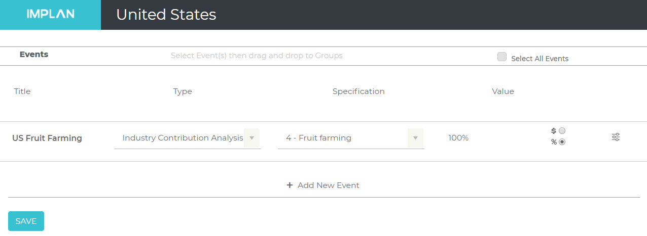
First, we create the region for US Total and enter the Impacts screen.  We start defining our Event by giving the Event a title like “US Fruit Farming.”  Under Type, we choose “Industry Contribution Analysis” and under Industry we choose “4 – Fruit Farming.”  

Under the Value field, there are two choices.  First, we can enter the dollar value of the sector that we want to model.  This would be useful if we want to show the contribution of one large farm in our study area that we know has an output of $2 million.  The other choice is a percent which is most useful when we want to model the contribution of the entire sector on the economy. In this example, the Value is set to 100% so that we can examine the contribution of all fruit farming across the nation.

The screen should look like this: 

contribution_event.png

Now, we move our Event into the Group on the right side of the screen.  Our Group will need to indicate the US Total as the Region. By default the Dollar Year will be the current year and the Data Year will be the most current data available in IMPLAN. These settings are appropriate for estimating the contribution of an entire Sector for the current year. Note that different years of data can be analyzed by manipulating the dollar year on the Events screen and these settings can be updated as appropriate. Now  we are ready to run our analysis. For our example, let’s estimate the contribution of fruit farming in 2017 for the whole US. 

STEP 2 – EXAMINE THE RESULTS

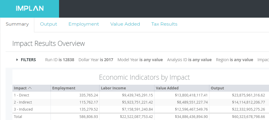
As always, the Results screen starts with a summary of the analysis.  Here we can see that the direct employment in Sector 4 -Fruit Farming is 335,765, the Labor Income is $9.4 billion, the Value Added is $13.8 billion, and the Output is $23.9 billion.  The total effect on the national economy is 586,806 jobs, $22.5 billion in Labor Income, $34.9 billion in Value Added, and $60.3 billion in Output.

contribution_results_summary.png

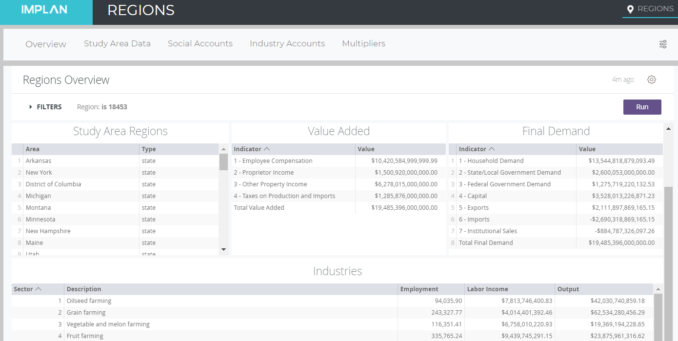
From our Region Details screen, there is a descriptive picture of the entire economy.  When examining the Industry Detail, we see the exact same Direct Employment, Labor Income, and Output shown in our Results of the fruit farming ICA.  This is because we chose to model 100% of the Sector and maintained a consistent Dollar Year in our analysis Events and Results, which also matches the year of the data.

contribution_overview.png

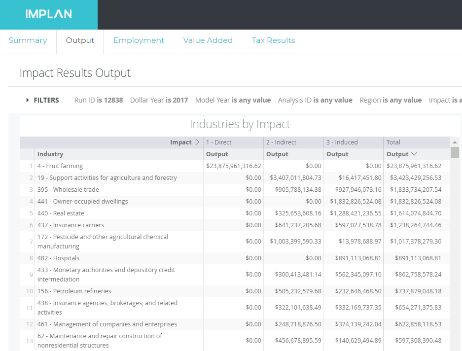
Moving to the Output tab, we can see that the Indirect and Induced effects for Sector 4 – Fruit Farming are zero.  This means the model did not allow any buybacks from the sector to itself. The same is true on the other tabs for Employment as well as all the components of Value Added (Employee Compensation, Proprietor Income, Other Property Income, Taxes on Production & Imports, and a total for Value Added).

contribution_detail_results.png

STEP 3 – THINKING THROUGH YOUR ANALYSIS

This method can also be done for just one business to see how perhaps one large farm contributes to a regional economy.  Remember, this is done by inputting only the dollars of output or percent of the total sector represented by that farm on the Events page, while still using the Industry Contribution Analysis type. This is definitely the conservative approach when a firm is small in the region in comparison to the remainder of the sector.

Industry Contribution Analysis can also be done across multiple sectors, for example to show how all of agriculture fits into the economy of study.  This is done by adding multiple Events as perhaps we also want to see vegetable farming or perhaps all agriculture sectors together.  Each sector would be its own Event as an Industry Contribution Analysis so we would see one Event for Sector 4 – Fruit Farming, another for Sector 3 – Vegetable and Melon Farming, etc.

If you model each of these Contribution Events for each Sector within a single Group, this will treat the analysis as a Multi-Industry Contribution Analysis, such that the purchases from a Sector to itself are restricted AND the purchases from other Sectors to the modeled contributing Sector are also restricted. This would produce results that only include Direct Effects for the Sectors included in your multiple Industry Contribution Analysis Events. All Indirect and Induced Effects to these Sectors would be restricted from being generated. If the Industry Contribution Analysis Events for each Sector were modeled within individual Groups, then each Group will be treated as a single Contribution Analysis where only the purchases from each Sector to itself are restricted. 


USEFUL TIP:

If you are performing an ICA on individual states and DC, and then the US total, the sum of the individual impacts will not match the national total.  This is true for any derivation of smaller groups (congressional districts, zip codes, counties) and one larger area because each region has a unique commuter rate and trade flows so the sum of the parts will never be the same as the total.  We recommend that you manually sum the totals from the smaller regions instead of using the results from the larger region if the you plan to present both sets of data in the same context.


CASE STUDY:

A $2.1B Apples to Apples Contribution Analysis in New York State 


WEBINAR:

Industry and Multi-Industry Contribution Analysis: A Primer, How-To Guide, and Best Practices 


RELATED TOPICS:

Considerations of Contribution Analysis – IMPLAN Online & IMPLAN Pro

ABP: Analysis-by-Parts with Manually Margining Bill of Goods

These instructions are an optional component of the Bill of Goods ABP approach

INTRODUCTION:

When you have a Bill of Goods (BOG) or line-item budget available in addition to your labor costs, you may want to create a spending pattern unique for your Industry using Analysis-by-Parts (ABP)

The Intermediate Expenditures that are purchased by the business can be modeled in several different ways. Intermediate Expenditures are determined and modeled by IMPLAN for Industry Events, but they can also be modeled separately as a part of an ABP analysis within an Industry Spending Pattern or on an individual basis as a Commodity Output Events.  

When Intermediate Expenditures are purchased via retail or wholesale venues, Margins become relevant and therefore using the Commodity approach may be more suitable. Since the prices paid to a wholesaler or retailer are purchaser prices and not producer prices, adjustments need to be made to the sales value.  


DETAILED INFORMATION:

ABP can be an incredibly useful technique for digging deeper into a firm’s budgetary expenditures, but when we look at retail or wholesale purchases, it is important that these purchases are handled carefully. The reason for this is that IMPLAN understands values only expressed in producer prices, but a retail or wholesale gross sales value (known as the purchase price) includes not only the production component of the retail or wholesale venue but also the production of all the elements of the Value Chain that proceed it. Thus, the gross sales value of a retail sale is a combination of the Retail Value, Wholesale Value, Transportation Value, and Producer Value. The wholesale gross sales value is actually a combination of the Wholesale Value, Transportation Value, and Producer Value. Thus, if we create a coefficient of spending for either a retail or wholesale component without Margining, or if we apply the entire value to the production Sector’s coefficient, we will be mis-estimating the impacts on those respective Sectors.

There are two possible situations that might arise:

  1. Purchases are known to be retail or wholesale, but the specific items purchased are unknown.
  2. Purchases are known to be specific items, but the value associated to them is a wholesale or retail gross sales value.

These two situations will be handled in the Usage section in two different examples using simplified spending as examples.


THE PROCESS:

Example 1: Retail or Wholesale Purchase Value Is Known, but the Item Purchased Is Unknown

A Kansas flour milling business, Best of Grains, buys supplies as part of its production function. We know that of their $15,000,000 Output value they spend $1,000 a year at the local Office Retail Superstore and $21,600 through a Wholesaler. Our first inclination might be to simply create coefficients based on the respective portions of the total cost that these purchases represent. If we were to do so, we would represent these coefficients as:

ABP_Margins_-_Table_1.jpg

However, this would be attributing too much value to the Retail and Wholesale Sectors involved.

In order to determine what the Margin should be for each of these Sectors, we need to adjust the sales value further by determining what portion is kept by the retailer and wholesaler respectively. Note that in this circumstance, because we do not know the items purchased, the value that cannot be attributed to the retailer or wholesaler is leaked from the spending pattern.

We will get the Margin value from the “2017 COMMON (IMPLAN5) MARGINS” spreadsheet. 

Column A: The Producer (in this case the producing Sector would be grains)

Column B: The Industries and Commodities available to receive component parts of the Value Chain (Retail Value, Wholesale Value, Transportation Value, and Producer Value). Note that while not all the Retail Sectors (369-407) have values in column C, they are all present.

Column C: The portion of the Total Sales value that goes to the Sector listed in Column B.  Also, the Retail and Wholesale Sectors (395-407) have the same Sector designation in Columns A and B.

For our example, we do not know exactly what is being purchased, so we are going to highlight Column A and use the Find function in Excel to search for 3395 – Wholesale Trade, as well as 3406 – Retail- Miscellaneous Retail Stores. You should see the portion of the table captured below:

ABP_Margins_-_Excel_Download_395.jpg

With this new information, we will now reformulate our coefficient calculation to include the Margined values captured from the spreadsheet above.

ABP_Margins_-_Table_2.jpg

Thus when we added these components to our spending they would be represented as their Margined coefficients.

Now we can enter the information with the rest of the Bill of Goods as shown here.

ABP_Margins_-_Event_Screen.jpg


Example 2: Item Purchased Is Known, but the Value Is Expressed in Retail or Wholesale Costs

Best of Grains also buys grain as one of the primary components of its production. Of their $15,000,000 annual Output, they spend $8,400,000 on grain, but they purchase the grain through a wholesale food provider.

Just like above, we cannot directly attribute the $8.4 million in production to Sector 2 – Grains. But unlike in Example 1, we know exactly what our flour mill is purchasing in this circumstance. But now there is also an added caveat. When we look at the splits for Sector 2, we see that all elements of the Value Chain are included in the spreadsheet: Margin splits for Retail Value, Wholesale Value, Transportation Value, and Producer Value. However, we know there is no retailer because the purchase was made through a wholesaler. We will need to recalculate the Margin splits by adjusting the provided values so that the portion of the Margin assigned to the retailer in the table is redistributed into the wholesale, transport, and production elements of the Margin.

ABP_Margins_-_Excel_Download_3002.jpg

To do this we will need to zero out the retail Margin and normalize the remaining Margin values. We can normalize the remaining Margins as follows:

ABP_Margins_-_Table_3.jpg

Now that we have adjusted the Margins to account for the entire sales value without the retail component, we can apply the Margin values to the grain purchase to determine how much of the grain purchase goes to each of the other respective Sectors.

ABP_Margins_-_Table_4.jpg

So now we split the Grain entry into the new margined pieces as shown here.

ABP_Margins_-_Event_Screen_Grain_Split.jpg

While this represents a simplified example, the same principles apply to Margining larger more complicated projects as well. Note that more than one component in a spending pattern will likely have Wholesale and Retail purchases. It is usually best, unless you want to create a single Event for each part of the Value Chain (retail, wholesale, transportation, production), to sum these coefficients on like Sectors (ie combining all the Wholesale) into their total component so you have only one Event for each.

Remember, in these cases Capital Expenditures should be modeled separately from any operations or construction of the business. 


ADDITIONAL CONSIDERATIONS:

What about the Local Purchase Percentage?

This should be set to SAM Model Value. This will allow the Model to make estimates of local purchasing ability of all Commodities. 

Thinking about Transportation

Typically there are two legs of transport: between the producer and the wholesaler and between the wholesaler and the retailer. The transportation expenses should be accrued into a single Sector. If you are using the IMPLAN Margin splits as outlined in this article, both legs of transportation are included in the respective Margin components.  Keep in mind, however, that the first leg could be via ship from the producer to the wholesaler, while the second leg is via truck from the wholesaler to the retailer. 

Zeroing out the Retail Margin

In this case, we re-normalized across all Margin Sectors to remove the retail component in Example 2. However, this is not the only option, though it is typically the most conservative one. In contrast, you could argue that the wholesaler and transporters do not get a larger cut when there is no retailer. Perhaps it is more likely that the producer gets to keep the difference or splits the difference with the wholesaler. You can make these adjustments based on what you know about the Industry, and then state how you handled the normalization process in your results.


RELATED ARTICLES:

ABP: Introduction to Analysis-By-Parts

ABP: Analysis-by-Parts & Bill of Goods Using Commodity or Industry Events with Labor Income Event(s)

ABP: Analysis-by-Parts Using an Industry Spending Pattern Event with Labor Income Event(s)

Hospitals: Modeling Private Hospital Impacts with Analysis-by-Parts

Hospitals: Modeling Public & Nonprofit Hospital Impacts with Analysis-by-Parts

Proving Analysis-By-Parts: A Comparison of Event Types

ABP: Analysis-by-Parts Using an Industry Spending Pattern Event with Labor Income Events

INTRODUCTION:

Analysis-by-Parts (ABP) is a technique by which you can split the “stemming ripple effects” of an event into its individual impact components. Separating the pieces with Analysis-by-Parts gives the researcher more flexibility and customization capabilities in the analysis. 


DETAILED INFORMATION:

To perform an Analysis-by-Parts, you will want to know Direct Labor Income and the Direct Intermediate Expenditures or Output, as well as the Industry that your business is best represented by. If Direct Labor Income, Intermediate Expenditures and Output are unknown, Output can be calculated using the Output-per-worker for the Sector that best represents your business or industry (Region Details > Study Area Data > Industry Summary, Output-per-Worker column, Sector row).  Hold onto this number, we’ll need it at the end. 

handy template is here for you to use as you follow along with this example.


ABP_-_Industry_Spending_Pattern_and_Labor_Income_-_Industry_Summary.jpg


When the Industry you are modeling doesn’t match IMPLAN’s Output equation for the Industry, Analysis-by-Parts is appropriate. Performing an Analysis-by-Parts using an Industry Spending Pattern is most commonly used when modeling a nonprofit or public organization, because these organizations do not typically allocate an equal portion of their Output to Tax on Production and Imports (TOPI) or Other Property Income (OPI) as for-profit, private businesses. This technique is also useful for modeling a more specific type of industry than available in IMPLAN according to the default 546 Industry scheme, but this requires editing of the Industry Spending Pattern and the information to do so. 

STEP 1 – EXPENDITURES

Intermediate Expenditures should be applied to an Industry Spending Pattern. These Industry Spending Patterns are made up of all the Commodities expected to be purchased by the Industry for annual operations. 

Create an Event for the Intermediate Expenditures first. Populate the Event with a Title that makes sense to you and for the Type, select 2018 Industry Spending Pattern. 

Let’s take for example, a new public university that will open in West Virginia.  Select the Industry that best represents your business in the Specification Field. In this case, it is Industry 481 – Junior colleges, colleges, universities, and professional schools.  However, this Industry represents private establishments. 

Now, we need to put together the Output equation.


Output___IE_EC_PI_TOPI_OPI.jpg


The Intermediate Expenditure Coefficient can be found as the Gross Absorption column total in 

Region Details 
     > Social Accounts 
          > Balance Sheets
               > Industry Balance Sheet
                    > Commodity Demand

For WV in 2018 this value is 38.714%.


ABP_-_Industry_Spending_Pattern_and_Labor_Income_-_Finding_IE.jpg


IMPLAN says the Output Equation for this Industry in WV in 2018 is: 

The addition coefficients for the components of Value Added can be found in the Value Added Coefficient column in:

Region Details 
     > Social Accounts 
          > Balance Sheets
               > Industry Balance Sheet
                    > Value Added


ABP_-_Industry_Spending_Pattern_and_Labor_Income_-_Finding_VA.jpg


We know Output is the sum of Intermediate Expenditures + Employee Compensation + Proprietor Income + Other Property Income + Taxes on Production and Imports. Therefore, these five numbers should add together to give you 100%.

Output (100%) = 

     Intermediate Expenditures (38.71%) + Employee Compensation (41.58%)
     + Proprietor Income (1.55%) + Other Property Income (12.68%)
     + Taxes on Production and Imports (5.47%)

The public university we are hoping to model does not have any proprietors and it is tax exempt. While the public university does not generate any profit, it still may have some OPI for consumption of capital, this could include things like a purchase of new computers for the library. Determining how your industry or business’s Output Equation differs from IMPLAN’s definition is up to you as the analyst. 

If you have your own information about spending on Intermediate Expenditures and Labor Income, this is ideal! Your Intermediate Expenditure value can be entered into the Event Value Field.

If you do not have the total spending amount on Intermediate Expenditures, you’ll need to calculate this using Output and your Industry’s Output Equation. 

To generate the Output Equation for the public university in our example, we need to remove PI and TOPI from our Output equation. We will do this by zeroing those out and renormalizing the equation.

First, we’ll need to sum the portions we want to keep:

     Intermediate Expenditures (38.71%) + Employee Compensation (41.58%)
     + Other Property Income (12.68%) 
     = 92.98%

Next, we’ll divide each portion we are keeping by the new total to get new portions summing to 100%:

     New Intermediate Expenditure portion: 38.71% / 92.98% = 41.64%
     New Employee Compensation portion: 41.58% / 92.98% = 44.72%
     New Other Property Income portion: 12.68% / 92.5% = 13.64% 

The value for Intermediate Expenditures can be calculated as Output * Intermediate Expenditure coefficient and entered in the Event Value field. If Output for the university is $5M, then Intermediate Expenditures for the public university equals $5,000,000 * 41.64% = $2,081,912.73.


 ABP_-_Industry_Spending_Pattern_and_Labor_Income_-_IE_Event.jpg


If you’d like to make any edits to this Industry Spending Pattern because some information about the universities operating expenses is known, you can do so by opening the Menu. 

This will open the following module where you can add Commodities (Arrow A), delete Commodities (Arrow B), edit the portion of Intermediate Expenditures going to a given Commodity (Arrow C), edit the Local Purchase Percentage LPP (Arrow D), and re-sum the Intermediate Expenditure coefficients to 100% by normalizing or convert back to the original settings by resetting (Arrow E). 


ABP_-_Industry_Spending_Pattern_and_Labor_Income_-_Advanced_Editing.jpg


Editing an Industry Spending Pattern can become cumbersome if you have a full detailed list of expenditures. To model these Intermediates Expenditures as individual Commodity or Industry purchases, follow the instructions for Analysis-by-Parts & Bill of Goods: Using Commodity or Industry Events with Labor Income Events


STEP 2 – LABOR INCOME

Next, a Labor Income Event must be created either for Employee Compensation (EC), Proprietor Income (PI), or both.

In our example, the university will only have wage and salary workers so the total payroll value at the university should be run through a Labor Income Event with the Specification of Employee Compensation. 

Remember, these should be fully loaded payroll values which include wage and salary, all benefits (e.g., health, retirement) and payroll taxes (both sides of social security, unemployment taxes, etc.).  

If you need to convert your wage and salary data to fully loaded payroll, use the file Convert IMPLAN 546 Employment to FTE and Income to EC 2018.

Let’s say in our example, payroll is unknown. We can calculate Employee Compensation by multiplying the university’s Output by the university’s Employee Compensation coefficient by taking Output $5,000,000 * 44.72% = $2,235,983.09.

ABP_-_Industry_Spending_Pattern_and_Labor_Income_-_2_Events.jpg


STEP 3 – RUN THE IMPACT

Now either use the button at the top to select all or highlight each Event and drag them into your Group.  Next, hit run.


ABP_-_Industry_Spending_Pattern_and_Labor_Income_-_WV_Group.jpg


STEP 4 – INTERPRET THE RESULTS

When your analysis is complete, the results will show you the economic impact of all of the Events you entered which will include the Industry Spending Pattern Event and the Labor Income Event.

In our public university example, the schools annual operations has Indirect and Induced impacts of approximately 19 jobs, $809,056 in Labor Income, $1.5M in Value Added, and $2.9M in Output.

  • Indirect Effects are from the Industry Spending Pattern Events only and represent activity in the local industries affected by Direct business’s supply chain.
  • The Labor Income events only create Induced Effects.


STEP 5 –  MODIFYING RESULTS

Because the spending by the Direct business was modeled instead of the Direct business itself, there is no Direct Effect in your Results. Using the information we found Behind the i and calculated, we can find the Direct Effects.

Define your Direct Effect:

  • We know Direct Output = $5M
    Also, IE + VA = Output

$2,081,912.73 + $2,918,087.27 = $5M

  • Direct Value Added = Employee Compensation + OPI (there is no PI or TOPI)
    $2,235,983.09 + $682,104.18 = $2,918,087.27
  • Direct Labor Income = Employee Compensation
    $2,235,983.09
  • Direct Employment
    Output/Worker = $72,279.89
    Output = $5M
    $5M / $72,279.89 = 69.18

handy template is here for you to use to calculate the Output equation and add back in your Direct Effects.


TEMPLATE:

ABP – Public University Institutional Spending Pattern & Labor Income Events

NAICS

IMPLAN's Core Data Release is now live! Current subscribers can automatically access the new data in-app. If you aren’t a subscriber, you can schedule a demo today to learn more about becoming one.

X