The Output Equation – Finding Values

INTRODUCTION:

All IMPLAN Industries have a unique Output Equation for each Region and Data Year. You may want to look Behind the i to see a specific Output equation. You can also use this data to find or calculate any part of the Output Equation: Output, Intermediate Expenditures, Value Added, Labor Income, Employee Compensation, Proprietor Income, Taxes on Production and Imports less Subsidies (TOPI), and  Other Property Income (OPI).


USING THE OUTPUT EQUATION:

Using the data in IMPLAN to figure out the missing pieces of the Output equation can be valuable if you are trying to find out what an Industry may spend on Intermediate Expenditures or the percent that is going to TOPI, for example. First, head Behind the i to Customize Region.


Output_Equation_-_Customize_Region.jpg

FINDING INTERMEDIATE EXPENDITURES

Let’s take a look at Industry 2 – Grain Farming at the U.S. level in 2018.

Output_Equation_-_2_Grain_Farming.jpg

IMPLAN reports Output, Employee Compensation (EC), Proprietor Income (PI), Other Property Income (OPI), and Taxes on Production and Imports less Subsidies (TOPI) along the left side of the box. The column on the right reports these values per worker (/w).

We know the formula for Output:

Output___IE_EC_PI_TOPI_OPI.jpg

And IMPLAN has shown us all but one of these values: Intermediate Expenditures. So we can figure that out by solving for the one missing piece.

$67,702,408,597  = IE + $3,606,890,353 + $6,841,169,324 + -$1,004,059,364 + $10,883,017,114

$67,702,408,597  = IE + $20,327,017,426

IE = $47,375,391,171


FINDING VALUE ADDED

Value Added is simply the summation of EC + PI + TOPI + OPI.  Again using Industry 2 – Grain Farming, we can find Value Added.

VA___EC_PI_TOPI_OPI.jpg

VA = $3,606,890,353 + $6,841,169,324 + -$1,004,059,364 + $10,883,017,114

VA  = $20,327,017,426


FINDING LABOR INCOME

Labor Income is simply the summation of EC + PI.  Again using Industry 2 – Grain Farming, we can find this value.


LI___EC_PI.jpg


LI = $3,606,890,353 + $6,841,169,324 

LI  = $10,448,059,677


RELATED ARTICLES: 

The Output Equation

The Output Equation – Differences by Industry

Output, Value Added, & Double-Counting

CEW Data

INTRODUCTION:

The 2018 Census of Employment and Wages (CEW) dataset is complete and now available to purchase in easy to use Excel files. Because of the level of detail and historic data available, the CEW data is perfect for establishing trends and running statistical analyses. The CEW data is useful for completing trend analyses and deep dives into U.S. wage and salary information. Drilling down into specified sector data allows for users to explicitly define the industry they wish to analyze at a granular level. 


PRODUCT DETAILS:

The Bureau of Labor Statistics collects a quarterly count of employment and wages across the U.S. called the Quarterly Census of Employment and Wages (QCEW). It uses data that is reported by employers covering more than 95% of jobs across the country. Data is then made available at the county, state, and national levels. 

The Bureau of Labor Statistics (BLS) releases CEW data, however there are certain non-disclosures within their data. The data contains employment, wages, and establishments in a given sector and area (down to the county level) and contains this information at the 6-digit NAICS level. This allows for even greater detail in specific modeling scenarios. IMPLAN adds value by filling in these non-disclosures based on existing data to be able to provide a complete picture.

The CEW data is available for 2001 to current IMPLAN data year (2018). IMPLAN refreshes these every five years as part of the panel data process, which is currently underway. The CEW data are for counties and up (including Puerto Rico and its municipios). The CEW data contains a Read Me file with additional information.


DATA DELIVERY & SUPPORT:

The data will be provided in .xlsx files containing the CEW data for the requested years. Users will have unlimited access to IMPLAN Community Forum at support.implan.com for questions specific to the data. IMPLAN economists will gladly respond to questions on IMPLAN’s Community forum within 5 business days at no additional charge. IMPLAN does not support data-application or related questions via email, phone, project consultation, or community forum.

To learn more about IMPLAN CEW Data, please contact IMPLAN at 800-507-9426 or sales@implan.com.


LICENSE AGREEMENT:

Access to the IMPLAN CEW Data is protected with a custom license agreement.  The license agreement will be presented when you are ready to purchase data. Sorry, the lawyers make us do it.


RELATED ARTICLES:

CEW FAQ


BLOG:

New CEW Data Available Now


WEBINAR:

Occupational Matrices: Occupational Employment and Compensation by Industry

2018 U.S. Territories Data Release Notes

INTRODUCTION:
IMPLAN has data for the five Island territories of the U.S. We have data on American Samoa (AS), Commonwealth of Northern Marianas Islands (MP), Guam, (GU), Puerto Rico (PR), and Virgin Islands (VI). Note that the data sets for Island Areas are not nearly as comprehensive nor timely compared to the U.S., unfortunately. The 2018 U.S. Territories data contain two significant additions.

2018 UPDATES:
PROPRIETOR EMPLOYMENT ESTIMATES
While prior U.S. territories data has included estimates of proprietor income (PI), proprietor employment was not included as part of a given industry’s employment value (unlike IMPLAN U.S. data). The decision to not include proprietor employment was a conservative one made due to a lack of data on U.S. territory proprietors. However, proprietor estimates, derived using U.S. level sector-specific rates of proprietors-per-PI, are included this year to promote definitional consistency with labor income, which includes both wage and salary income and proprietor income.

Employment overall is up, which is expected with the inclusion of proprietor employment. Those sectors seeing the largest jump in employment will be those with a higher rate of proprietors-per-PI at the U.S. level, which generally equates to those sectors with a larger proportion of proprietor employment (e.g., agriculture sectors, personal services sectors, etc.).

IMPROVED GOVERNMENT SECTOR DISTRIBUTIONS
U.S. Territories data now mimics IMPLAN’s domestic data production in the use of BLS CEW ownership codes to derive government employment and wages data for IMPLAN sectors beyond just administrative payroll for education and non-education. For Puerto Rico (PR) and Virgin Islands (VI), both of which are covered by CEW, ownership code data provide employment and wage data for additional government activities such as passenger transit, electric utilities, and other government enterprises, along with continued employment and wage data for government administrative sectors. For territories lacking BLS CEW coverage, PR and VI CEW data are used to estimate these new distributions of total non-education government employment and wages between non-education administrative government and the government enterprise sectors (passenger transit, electric utilities, and other government enterprises).

With the 2018 data, you will now see non-zero estimates for government sectors that were previously zero. These include passenger transit, electric utilities, and other government enterprises.

DATA DELIVERY & SUPPORT:
U.S. Territories data is utilized only in IMPLAN Pro and provided in .odf form (i.e., similar to international models, but the U.S. Territories data utilizes the same Structural Matrix as the domestic data). No Journey to Work (JTW) or Trade Flow files are included. The Industry scheme is identical to that used for IMPLAN Pro domestic data and contains 544 Industries.
To learn more about our data on U.S. Territories, please contact IMPLAN at 800-507-9426 or sales@implan.com.

Canadian Data Products

IMPLAN has released the 2012 Canadian Total File as well as Provincial level data. These IMPLAN data sets are based on the 2012 Statistics Canada data and have 103 sectors. Updated data at the national level is available using OECD data (rather than based on StatCan data.)

The Canadian data sets are not able to be aggregated, as each Provincial data file has a separate Structural Matrix. Each Province needs to have a separate model built. The current Canadian Provinces are not MRIO compatible for the same reason that the regions are not able to be aggregated.

While the data files are not downloadable, once your order is placed an IMPLAN support agent will call you to arrange the transfer of the data files.

CANADIAN PROVINCIAL LEVEL DATA
Alberta British Columbia
Manitoba Yukon
Saskatchewan Newfoundland
New Brunswick Northwest Territory
Quebec Nunavut
Nova Scotia Ontario
Prince Edward Island

SECTOR DESCRIPTIONS
Crop and Animal Production Forestry and Logging Fishing, hunting and trapping Support activity for agriculture and forestry
Oil and gas extraction Coal mining Metal ore mining Non-metallic mineral mining and quarrying
Support activities for mining and oil and gas extraction Electric power generation, transmission and distribution Natural gas distribution, water, sewage and other systems Residential building construction
Non-residential building construction Engineering construction Repair construction Other activities of the construction industry
Animal food manufacturing Sugar and confectionery product manufacturing Fruit and vegetable preserving and specialty food manufacturing Dairy product manufacturing
Meat product manufacturing Seafood product preparation and packaging Miscellaneous food manufacturing Soft drink and ice manufacturing
Breweries Wineries and distilleries Tobacco manufacturing Textile and textile product mills
Clothing and leather and allied product manufacturing Wood product manufacturing Pulp, paper and paperboard mills Converted paper product manufacturing
Printing and related support activities Petroleum and coal product manufacturing Petroleum and coal product manufacturing Resin, synthetic rubber, and artificial and synthetic fibers and filaments manufacturing
Pesticide, fertilizer and other agricultural chemical manufacturing Pharmaceutical and medicine manufacturing Miscellaneous chemical product manufacturing Plastic product manufacturing
Rubber product manufacturing Non-metallic mineral product manufacturing (except cement and concrete products) Cement and concrete product manufacturing Primary metal manufacturing
Fabricated metal product manufacturing Machinery manufacturing Computer and peripheral equipment manufacturing Electronic product manufacturing
Electrical equipment and component manufacturing Household appliance manufacturing Motor vehicle manufacturing Motor vehicle body and trailer manufacturing
Motor vehicle parts manufacturing Aerospace product and parts manufacturing Railroad product and parts manufacturing Ship and boat building
Other transportation equipment manufacturing Furniture and related product manufacturing Miscellaneous manufacturing Wholesale trade
Retail trade Air transportation Rail transportation Water transportation
Truck transportation Transit, ground passenger and sightseeing, and support activities for transportation Pipeline transportation Postal service and couriers and messengers
Warehousing and storage Motion picture and sound recording industries Radio and television broadcasting Publishing, pay/specialty services, telecommunications and other information services
Depository credit intermediation and monetary authorities Insurance carriers Lessors of real estate Owner-occupied dwellings
Rental and leasing services and lessors of non-financial intangible assets Other finance, insurance and real estate services and management of companies and enterprises Legal, accounting and architectural, engineering and related services Computer systems design and other professional, scientific and technical services
Advertising, public relations and related services Administrative and support services Waste management and remediation services Educational services
Health care and social assistance Arts, entertainment and recreation Accommodation and food services Repair and maintenance
Personal services and private households Professional and similar organisations Non-profit education services Non-profit social assistance
Non-profit arts, entertainment and recreation Religious organizations Miscellaneous non-profit institutions serving households Public educational services (except universities)
Public universities Public hospitals Public nursing and residential care facilities Other federal government services
Other provincial and territorial government services Other municipal government services Other aboriginal government services

International OECD Data Sets

INTRODUCTION:
IMPLAN now has data for the Organization for Economic Co-Operation and Development (OECD) countries. IMPLAN OECD data covers 35 countries with 37 Industries and corresponding Commodities. The model is created based on OECD 2015 Input-output table at basic prices.

Final Demand includes:

Final consumption expenditure of households
Final consumption expenditure of non-profit institutions serving households (NPISH)
Final consumption expenditure of general government
Gross fixed capital formation
Changes in inventories
Value added components include:

Employee Compensation
Net Taxes on Products
Gross Operating Surplus
Other Taxes less than Other Subsidies on Production

OECD COUNTRY LIST:
Argentina Colombia Korea Saudi Arabia
Australia Costa Rica Malaysia Singapore
Brazil Hong Kong Mexico South Africa
Brunei Darussalam Iceland Morocco Switzerland
Cambodia India New Zealand Thailand
Canada Indonesia Norway Tunisia
Chile Israel Peru Turkey
China Japan Philippines Vietnam
Chinese Taipei Kazakhstan Russian Federation

LIST OF INDUSTRIES:
Agriculture, forestry and fishing Fabricated metal products, except machinery and equipment Telecommunications
Mining and extraction of energy producing products Computer, electronic and optical products IT and other information services
Mining and quarrying of non-energy producing products Electrical equipment Financial and insurance activities
Mining support service activities Machinery and equipment n.e.c. Real estate activities
Food products, beverages and tobacco Motor vehicles, trailers and semi-trailers Other business sector services
Textiles, wearing apparel, leather and related products Other transport equipment Public administration and defense; compulsory social security
Wood and of products of wood and cork (except furniture) Other manufacturing; repair and installation of machinery and equipment Education
Paper products and printing Electricity, gas, water supply, sewerage, waste and remediation services Human health and social work
Coke and refined petroleum products Construction Arts, entertainment, recreation and other service activities
Chemicals and pharmaceutical products Wholesale and retail trade; repair of motor vehicles Private households with employed persons
Rubber and plastics products Transportation and storage Intermediate Taxes on Products
Other non-metallic mineral products Accommodation and food services
Manufacture of basic metals Publishing, audiovisual and broadcasting activities

To learn more about this data, please contact IMPLAN at 800-507-9426 or sales@implan.com.

Trade Flow Data

INTRODUCTION:
Have you ever wanted to take a peek at IMPLAN’s Trade Flow data? Have you been curious about the details of IMPLAN’s Gravity Model and Trade Flow RPCs? Then this might be the place for you!

IMPLAN’s domestic Trade Flow data set is comprised of county-to-county dollar values of domestic trade in all IMPLAN commodities (including services). The data are estimated via a doubly-constrained gravity model. The trade captured by this dataset is for both intermediate and final uses, and includes trade within a county (a county to itself). Cool right?

PRODUCT DETAILS:
The gravity model was originally adapted from Newton’s Law of Gravity! This law states that the attraction between two masses is directly related to the size of the masses and inversely related to the distance between them. The gravity model was first suggested in an I-O context in Leontief and Strout (1963). In the last fifty years, the gravity model has been widely used to predict trade flows (Federal Highway Administration, 1977, p. 118; Anderson and van Wincoop, 2003; Anderson, 2011).

In 2005, IMPLAN, in concert with the U.S. Forest Service, developed a sophisticated doubly-constrained (until all supplies go somewhere and all demands are fulfilled) gravity model to estimate trade flows for all IMPLAN commodities between all counties in the U.S. These Trade Flows show the movement of goods and services between and within counties or user-defined regions made up of counties. .

A key aspect of the data set is that the trade is on an origin-of-production basis, not an origin-of-movement basis. This means that the data set tracks from where a Commodity is produced to where it is consumed as either an intermediate or final use rather than from where a Commodity begins its export journey.

DATA SOURCES:
Each year, the IMPLAN database is used to create the attracting masses (supply and demand) for each U.S. county and each Commodity. These county masses are combined with distances (cost of transport indexes) between and within counties by mode of transport from Oak Ridge National Laboratory’s (ORNL) Transportation Network. The model is calibrated using distances traveled by Commodity from the most recent Commodity Flow Survey (CFS).

DATA DELIVERY & SUPPORT:
Data is delivered as a SQL .bak file or a .csv file. These files contain a single table with all county-county pairs and all Commodities. In this table, the counties are indexed from 1 to 3141 with no associated FIPS codes. A bridge table is included to match the county index to the appropriate FIPS code.

READY TO MODEL:
To learn more about purchasing our Trade Flow data, please contact IMPLAN at 800-507-9426 or sales@implan.com.

RESOURCES:
Anderson, J.E. and E. van Wincoop. 2003. Gravity with Gravitas: A Solution to the Border Puzzle. The American Economic Review, 93(1): 170- 192, March.

Anderson, J.E. 2011. The Gravity Model. Annual Review of Economics, Volume 3: 133-160.

Commodity Flow Survey (CFS)

Federal Highway Administration. 1977. Computer Programs for Urban Transportation Planning.

IMPLAN’s Gravity Model and Trade Flow RPCs

Leontief, W. and A. Strout. 1963. “Multiregional Input-Output Analysis.” In Barna (ed.), Structural Interdependence and Economic Development, London: Macmillan (St. Martin’s Press), pp. 119-149.

Oak Ridge National Laboratory (ORNL)

Environmental Data

INTRODUCTION:

IMPLAN has three core values: community, respect, and stewardship. The goal of being good stewards has taken us beyond examining only the economic impacts associated with changes in production to examining some of the environmental impacts associated with current and projected levels of production. Working with the U.S. Environmental Protection Agency (EPA), IMPLAN has bridged their emissions data to our Industries, thereby tying economic impacts to environmental impacts!  


PRODUCT DETAILS:

IMPLAN’s environmental data consist of Industry-specific coefficients of physical emissions or resource use per dollar of Industry Output. These ratios can be applied to the IMPLAN modeling system in order to gain insight into the environmental impacts associated with economic impact scenarios. The data also allows for the comparison of environmental footprints across geographies or over time.

The coefficients are Industry-specific, but the EPA data have somewhat less Industry-specificity than the IMPLAN data, such that some EPA ratios are mapped to more than one IMPLAN Industry.  In other words, some IMPLAN Industries have the same coefficients . 

The coefficients do not double count in that they do not include the emissions associated with the upstream industries/suppliers. For example, the emissions associated with the car manufacturing Industry do not include emissions associated with the production of car parts or other inputs produced by other Industries; the emissions associated with producing those inputs would be accounted for in the coefficients for those suppliers’ respective Industries. 

Any emissions generated directly by households (those not accounted for by household expenditures on electricity and not associated with the production of other items purchased by households) – for example, emissions generated by households’ burning of wood in a wood-fired stove in the home – are not included in the EPA dataset. Therefore, they are not accounted for in the IMPLAN emissions data set.  What this means is that all induced emissions in IMPLAN stem from household purchases of energy and of goods and services, all of which require energy to produce and thus create emissions. Any additional emissions generated directly by the household, those not associated with a purchase of energy, goods, or services, will not be accounted for.  

The coefficients are national-based.  The EPA is working on state-level data, which we plan to incorporate into subsequent iterations of the IMPLAN environmental data. Stay tuned.


DATA SOURCE:

IMPLAN’s environmental ratios are sourced from the U.S. EPA’s Environmentally-Extended Input-Output model (EEIO) data and the methodology put forth by Yang, Ingwersen, Hawkins, Srocka, and Meyer (2017). The data represented falls into 8 broad categories. Within these categories, tags are assigned to represent more specific types of each category. 

The categories are:

  • Criteria Pollutants
    • 267 tags
    • Examples: Nitrogen Oxides, Chromium III, Cellosolve Solvent
  • Greenhouse Gas Emissions
    • 15 tags
    • Examples: CO2, N2O, CH4, CF4
  • Land Use
    • 220 tags
    • Examples: Urban Land, Urban Transportation, Rural Transportation, Coal Exploration Licenses
  • Mineral Use
    • 5 tags
    • Examples: Boron, Gypsum, Salt
  • Nitrogen and Phosphorus Release to Water
    • 2 tags
    • Includes: N and P
  • Pesticide Emissions
    • 747 tags
    • Examples: Spirodiclofen/air, Norflurazon/water, Fluxapyroxad/groundwater
  • Toxic Chemical Releases
    • 408 tags
    • Examples: 1,2-Dichloropropane, 1,2-Phenylenediamine, 1,3-Butadiene
  • Water Use
    • 247 tags
    • Examples: Alpacas; On-farm surface source, Alpacas; surface water, Aquaculture; groundwater


DATA DELIVERY & SUPPORT:

Until the data are available in the IMPLAN application, the data will be provided in a .csv file containing the coefficients for each IMPLAN Industry. To analyze an environmental impact, one would take the industry Output figures from IMPLAN and multiply them by the coefficients from the environmental data. It’s as easy as that.

Users will have unlimited access to IMPLAN Community Forum at support.implan.com for questions specific to the bridging of the EPA data to IMPLAN Industries.  We can also refer users to the EPA for any questions regarding the calculation of their coefficients. IMPLAN economists will gladly respond to questions on IMPLAN’s Community forum within 5 business days at no additional charge. IMPLAN does not support data-application or related questions via email, phone, project consultation, or community forum.


LICENSE AGREEMENT:

Access to the IMPLAN Environmental Data is protected with a custom license agreement.  The license agreement will be presented when you are ready to purchase data. Sorry, the lawyers make us do it.


SAMPLE DATA:

Sample Environmental Data


GO GREEN:

To learn more about our environmental data, please contact IMPLAN at 800-507-9426 or sales@implan.com.


RESOURCES:

Ingwersen, W. An Introduction to USEEIO. The Strategic Analysis team for the Advanced Manufacturing Office, Cincinnati, OH, December 06, 2018. 

Yang, Y., W.W. Ingwersen, T.R. Hawins, M. Srocka, and D.E. Meyer, 2017. USEEIO: A new and transparent United States environmentally extended input-output model. Journal of Cleaner Production, 158: 308-318.

546 Industry Scheme

INTRODUCTION:

The 2018 data is now the default year in IMPLAN! The data release this year is especially exciting because we have a brand new Industry scheme with 546 Industries based on the updated BEA Benchmark and Census of Agriculture.

The new Industry scheme obviously has some changes from the 536 Industry scheme. We only lost three Industries due to disaggregation. Notably, wholesale trade has been split into 10 different wholesale Industries. Insurance carriers is now split into direct life and all others. Real estate is now split into tenant-occupied and other real estate. Finally, at both the local and state levels, the non-education spending pattern will be split into hospitals and health services and other services. Details on the changes can be found in the article BEA Benchmark & The New 546 Industry Scheme.


COMPARING DATA ACROSS TIME:

Compare data across time (2001 – 2018) in IMPLAN, using the most up-to-date Industry Scheme!

When there are significant changes to the underlying data, there is no longer an apples to apples comparison. Therefore, you will not be able to compare data sets, Projects or Event Templates in the 536 Industry scheme (or another) non-546 Industry scheme) with the new 546 Industry scheme. 

For comparing across different Industry Schemes, we have a bridge that should help in most instances. 

The 2018 data and the 546 Industry Scheme is the default on your Regions screen. The Regions screen will show you data from 2001-2018 in the 546 Industry Scheme. 

time_series.png


FINDING OLDER DATA:

To find the older data years (2012-2017), navigate from your home screen to the Projects screen.  On the Projects screen, click the NEW PROJECT button in the upper right.


New_Project.jpg


In the pop-up box, give your new Project a title and then in Industry Set, choose “US – 536 Sectors.” Then ensure that your Household Set is “Set 1 – (2015 Datasets or later).” This will give you the choice on your Regions screen between 2015, 2016, and 2017 datasets.  To find data from 2012-2014, choose “Set 2 – (2014 Datasets or earlier).”


 546_Sectoring_Scheme_-_Finding_2017.jpg


Click CREATE PROJECT and you will be taken to your Regions screen to set up as always!


New_Project_-_Create_Project_Button.jpg


RELATED TOPICS:

2018 Data Release Notes

546 Industries, Conversions, Bridges, & Construction – 2018 Data

BEA Benchmark & The New 546 Industry Scheme

Taxes: Industrial Breaks

INTRODUCTION:
Examining tax breaks, tax credits, tax exemptions, and tax incentives for firms and Industries is common in IMPLAN. This article outlines the basics on how you can use IMPLAN to examine the changes in your regional economy when tax policy affects Industries.

TAX BREAKS:
Tax breaks for certain Industries are common across the U.S. Municipalities offer huge tax incentives for site selection decisions or to encourage growth in basic Industries. Most times, these are in the form of foregone taxes; reducing the amount of future payments that would be required.

Even if the Direct taxes aren’t collected because of the incentive, there are still Indirect and Induced taxes generated because of the new activity. Showing the ripple effect of the government investment helps bolster support from taxpayers and justify the spending (or lack of tax collection). The return on investment (ROI) can be estimated using IMPLAN.

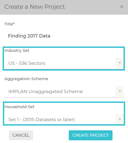
Let’s say for example, the state of North Carolina is going to give a complete Tax Exemption for 5 years to a new banking enterprise of the McDuck family. Their business plan estimates sales of $20M each year. We can run an Industry Output Event for $20M in Industry 441 – Monetary authorities and depository credit intermediation. Taking a look at the Tax Impact Results for the state, we see that Direct Taxes are reported. Now we know that they won’t be paying any Direct Taxes, so we can set our Filter to only show us Indirect and Induced Tax Results.

Tax_Breaks_-_Filtering_Indirect_and_Induced.jpg

Scanning down the screen, we see that because of the state investment which allowed for the resulting business to open in the state, North Carolina will see an additional $316,038 in Indirect and Induced Taxes in 2020. The state would not see the $325,106 of Direct Taxes in the first five years, but in year six, they would start seeing those revenues as well. If the argument can be made that but for the exemption, the McDuck family would have chosen another state for their bank, then it seems like it would have a positive effect on the state coffers; not to mention all of the sub-state level governments that will be collecting taxes.

Sometimes, however, businesses are given direct payments from the government to increase production, hiring, etc. These can be modeled through standard Industry Events in IMPLAN as new Output to the Industry.

Keep in mind that the distribution of the TOPI is based on the average of all Industries for you Region. If there is nothing unique about the tax structure of the business you are studying, then the resulting estimates are appropriate. However, if you are modeling a change in an Industry that will pay a higher share of a certain type of tax, it is best to edit your Direct Results to show that higher rate; IMPLAN will only show an average across all Industries. So if you are modeling Andrew’s Bootleg, a new distillery, and you know they will pay an additional sin tax or excise tax based on your local laws, it is best to use your estimate of the Direct Tax, and then use the Indirect and Induced tax results from IMPLAN.

TAX CHANGES:
Tax changes that affect an Industry vary widely; perhaps a new tax on production or inventory, new licensing requirements, etc. Analyzing these tax changes in IMPLAN depends on what the market reaction of the businesses will be. Will the business close, layoff employees, cut production, or see smaller profits? This determination is up to the analyst. Generally with a corporate tax increase, the first thing you will see is a reduction in corporate profit (OPI). In Input-Output models, corporate profit is treated as leakage as there is no way to know exactly how and where those profits are used as they could be reinvested in production, used for capital purchases, pay for additional hiring, distributed to shareholders, etc.

If the tax burden is so great as to force some businesses to reduce production, relocate, or close, this is an impact that could be modeled in IMPLAN. A simple Industry Output Event in the affected Industry could show the losses to the economy because of the new tax forcing out a local business.

OPPORTUNITY COSTS:
Another way IMPLAN can be used in examining tax issues is by looking at the Opportunity Costs – the benefit that is gained when one choice is made over another. Perhaps incentivizing the banking Industry would yield a smaller tax impact than the same dollar amount invested in automobile manufacturing. Not only can comparing these two potential scenarios show you the differences in how each affects the Regional economy of study but it will also show the differences in potential tax revenue.

EDITING TAX RESULTS:
You may have more specific knowledge about specific Direct Taxes that you want to adjust with the IMPLAN Results. Here’s how to do it.

Let’s say we have a plastics manufacturing firm that has chosen to remain in New Jersey due to the state’s offer to exempt them from Property Tax. We can run an Industry Output Event for their $5B in sales in 2020 in Industry 193 – Other plastics product manufacturing. On the Tax Results screen, Filter for the Direct Tax as the tax exemption is only being offered to the Direct business, and therefore Direct Tax is the only piece that will not be fully paid. Click on the ellipses to download the State Tax Impacts. Then click the download button and open up your Excel file.

Tax_Breaks_-_State_Tax_in_IMPLAN.jpg

Zooming in on the Property Tax, we see that there was a payment from Tax on Production and Imports (column) to TOPI: Property Tax (row) in the amount of $6,379.05. This would be the amount the state of NJ is giving up in Property Taxes.

When this data is in Excel, you can delete the $6,379.05 TOPI: Property Tax value from cell E7. You will need to recalculate the sum for Column E to show the new total as well as the sum of the Property Tax row in Column P and the sum of Column P itself to reflect the change. The new total for all of the Direct Taxes in NJ is $55,507,169. You can replace the original Direct Tax Figure with this new, lowered amount that will be collected by the State of New Jersey.

Tax_Breaks_-_Zero_Prop_Tax_in_Excel.jpg

You can Filter for the Indirect and then the Induced Taxes to see the amounts paid at the state level in order to calculate the total state taxes.

Tax_Breaks_-_New_State_Total_Tax_in_Excel.jpg

This process can be used to zero out or change any of the Direct Taxes on the IMPLAN results. For instance, you may know exactly how much a certain business will pay in a certain tax. Or perhaps you’d like to use your Industry-specific tax knowledge to shift around the distributions of TOPI or OPI in your Direct Tax results to compensate for the limitation in IMPLAN’s data on industry-specific tax distributions as mentioned in the Taxes: The Basics of the Breaks article. Use your bona fide knowledge of your subject to override the estimated Direct tax results in IMPLAN.

Taxes: Individual Breaks

INTRODUCTION:
If you haven’t already, check out the introductory article Taxes: The Basics of the Breaks to give you some general knowledge on tax breaks. Now let’s dive into some common tax breaks that individuals and households see and how to examine these in IMPLAN.

LABOR INCOME VS HOUSEHOLD INCOME:
There are two choices to model changes going straight to taxpayers in IMPLAN: Labor Income and Household Income. Let’s first look at the difference between Labor Income Household Income as illustrated below.

Tax_Breaks_-_LI___HI.jpg

Labor Income Events include all new labor payments including payroll tax, personal tax, and savings, as well as any labor payments to in-commuters who are local workers to the Region, but are not residents.

Household Income differs from Labor Income as it does not include the payroll tax paid on Labor Income nor does it include payment to workers that don’t live in the Region. Household Income does include personal taxes and savings. For Household Income Events, IMPLAN will not remove payroll taxes, social insurance taxes, or commuter spending, but will still remove personal taxes and savings.

When a Labor Income or Household Income Event is used, IMPLAN will calculate the leakages of income and the portion of income that is Household Spending based on the SAM. For further information check out the article on the Summary Description of Elements of the SAM.

ASSISTANCE PROGRAMS:
There are many government programs aimed at helping people from housing vouchers to encouraging the use of energy efficient appliances. As the analyst, you will have to decide which income categories will receive the benefit when using a Household Income Event and model them accordingly. For example, child care assistance is likely alloted to lower income earning categories.

For some tax breaks income level is not relevant; for example a tax refund for all taxpayers across the board. These kinds of tax rebates are not taxable, so they should be modeled through a Household Income Event. One caution when modeling these, however, is that while some of those receiving the benefit will likely spend all of it, some may put the refund into savings (and therefore should be omitted from the model). You can find the average savings rate by looking Behind the i in

Social Accounts >

IxC Social Accounting Matrix >

Detail IxC SAM

Then scroll to line 180 – Capital – Borrowing or Saving. You can divide the amount shown for each Household Income group by the total for that Household Income groups column to get an effective savings rate for each group. Note you will usually only see savings at higher earning levels.

To model the impact of a change in a specific program like Supplemental Nutrition Assistance Program (SNAP) benefits, there are two routes. The first option is to run increased spending through the main affected Industry; in this case 406 – Retail – Food and beverage stores. This assumes that this money will only stimulate the economy in terms of food purchases. However, you could also assume that the assistance allows families to have more money across various spending categories now that their food costs are being covered. In this case use a Household Income Event and analyze increases to only the income levels that will receive the benefit. Note that this method will still include spending on food.

CAPITAL INVESTMENTS:
Many municipalities offer tax breaks for the purchase of items like solar panels or energy efficient appliances. The reduction in the price of the item can be modeled with appropriate assumptions noted. The lowered price for the capital purchase could mean an increase in disposable income which can be modeled through a Household Income Event. However, the lowered price could just mean more money is moved into savings and has no impact.

You can also consider an increase in demand for capital items if they are manufactured in your study area. Perhaps the lowered price will incentivize more individuals to use the program and therefore purchase the required equipment. If this equipment is produced in your Region, you could model the increased sales of the manufacturing facility.

PROPERTY TAXES:
Property Taxes paid by Households are not displayed as a payment from Households; but rather from the TOPI column because Households pay Property Taxes on their home through Industry 449 – Owner-occupied dwellings. You can find the Property Taxes paid in your Region by looking Behind the i in

Social Accounts >

IxC Social Accounting Matrix >

Detail IxC SAM

Column 8001 – Taxes on Production & Imports makes a payment to line 159 – State/Local Govt Other Services – TOPI: Property Tax. The Property Taxes shown as being paid by Households are for other big-ticket items such as boats and cars.

As with modeling any type of tax break that affects individuals, you will have to make assumptions. For example, what would an increase in Property Taxes look like in your Region? Would that mean less disposable income (negative Household Income Event) or less in savings? Might some people even leave the Region in the face of an egregious rate hike?

SALES TAX:
Examining changes in Sales Tax rates depends again on what assumptions are being made about changes to spending within the Region. For a Sales Tax increase, the most basic level would be a negative Household Income Event showing less disposable income that can be spent due to the higher Sales Tax rate. However, be careful. If the county next door has a significantly lower tax rate, some of the shoppers from your county will likely head into the county with lower Sales Tax for bigger shopping days. This could mean decreased sales across retail Industries in your county. It could potentially mean the loss of some retail establishments in your Region.

If you wanted to look at Sales Tax that would be generated because of new employees in the Region, you can model the new employment through the appropriate Industry and check out your Results. The total tax impacts reported are those generated from the Event you ran. Filtering for the Induced Impact on the Tax Results screen will show the TOPI: Sales Tax stemming the household spending of the new employees and those working in Industries supported by your initial change. You could then estimate a per employee Sales Tax figure for your impact by dividing the Induced Sales Tax by the Direct + Indirect employment.