Location quotients (LQ) compare the relative concentration in a specific area to the concentration in the U.S. They are mainly used for descriptive and comparative purposes. The formula is LQ = Local Concentration / National Concentration, or more specifically the formula for the Employment LQ is:
LQ ir = (xir/xr) / (xin/xn)
where
xir = employment of sector i in region r
xr = total employment in region r
xin = employment of sector i in the reference region
xn = employment in the reference region
Typically, the reference region is the country in which region r resides, but it might also be a state or regional level. LQs can also be calculated using Output or Labor Income instead of Employment.
An LQ equal to 1 signifies that the local share is equal to the national share. An LQ of less than 1 means that the local share is less than the national share. An LQ of greater than 1 means the local share is greater than the national share and is typically an exporter or perhaps has a specialization in that Industry.
According to Bloomberg New Energy Finance, more than half of the cars produced by 2040 could be electric. This poses a huge change for traditional gasoline combustion engine production that has dominated the U.S. landscape. Currently, electric vehicles make up only a small portion of the market, representing only 3% in 2020. Because this industry is both relatively new and still small, it isn’t represented well in the automobile manufacturing industry.
PRODUCTION
The production of new vehicles of any type will fall under Industry 340 – Automobile manufacturing, 341 – Light truck and utility vehicle manufacturing, and 342 – Heavy duty truck manufacturing. However, these will be based on the status of the total Industry in the Data Year. That means that it includes all types of vehicles regardless of engine type.
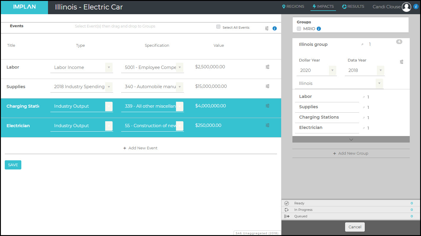
The best way to model the production of new electric vehicles is using Analysis-by-Parts (ABP). To use ABP, you would need to know detailed spending. Let’s take a look at an example of a new facility that will be built in Illinois by Varnado Motorcars, which will produce electric automobiles. We know they will spend $2.5M on labor and $15M on supplies. We also know that a full 5% of their supply spending will be on batteries sourced from within Illinois. So we will set up one Labor Income Event for $2.5M and one Industry Spending Pattern Event for $15M. Because Varnado Motorcars is a corporation, the $2.5M of Labor Income is all Employee Compensation earned by Wage and Salary workers. For our Industry Spending Pattern, we’ll specify the Industry most similar to the facility opening, Industry 340 – Automobile manufacturing, and then make the appropriate modifications.
Because we are told that 5% of the spending on Intermediate Inputs from local supplier Garrett’s Gadgets on batteries, we can open up the spending pattern to make the change.
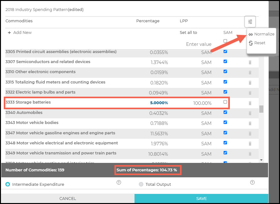
Scroll down to Commodity 3333 – Storage Batteries and change the given percentage to represent the 5% that will be spent on batteries from Garrett’s. Then unclick the SAM setting the LPP to 100% as we know these batteries will be sourced from Illinois. You can see the total sum of percentages is now 104.73%. To reset this to 100%, click Normalize in the upper right. Learn more about editing Industry Spending Pattern Events for other necessary changes, such as deleting Commodities not purchased as an Intermediate Input for electric vehicle manufacturing or adding Commodities that are unique to the electric vehicle production process.
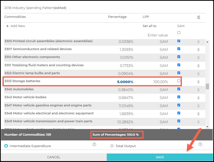
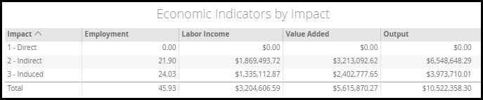
Now the sum of percentages is 100%. Click Save, Drag and Drop the 2 Events into the Illinois Region, and Run your Impact. With just a Labor Income Event and an Industry Spending Pattern Event in this ABP analysis, we have no Direct Effects in our Results.
To calculate our Direct Effects of Varnado Motorcars, the only other piece of information we need is Output/worker, which can be found:
Then we can use the Excel template to calculate the Direct Effects.
If this facility is being built instead of a traditional automotive plant, you might consider the opportunity cost of a combustion engine plant not being built. If the new facility is replacing the demand for combustion engine cars which may cause an old manufacturing plant to close, consider a Net Analysis to show how the electric vehicle production facility will differ from a combustion engine manufacturing facility.
CHARGING
In terms of construction of charging stations, if you don’t have the necessary details to conduct an ABP, the construction would fall under Industry 55 – Construction of new commercial structures, including farm structures. The operations of those facilities would usually fall under Industry – 408 Retail – Gasoline stores or whatever business is operating the station. If you have detailed information, however, ABP is suggested as this type of construction and operations represents such a small portion of these Industries in the current data and therefore any details you have on specific spending will yield a stronger analysis.
Charging stations do not take a lot to set up for operations. Treehugger notes that an electrician can install the unit and then it’s ready to go. Some of these charging stations are built in the U.S. and if they are being sourced from within your Region, this can be modeled as an Industry Event in 339 – All other miscellaneous electrical equipment and component manufacturing. Coupling this with associated costs to a local electrician in Industry 55 will round out the impact for installing charging stations. Here we see the addition of $4M in charging stations and $250K in electrician installation costs.
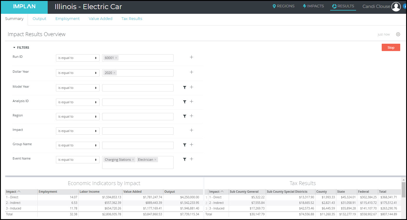
After running the analysis with these additional Events added to the Illinois Group, use the Filter on the Results screen and choose only the Charging Station and Electrician Events and click Run to see the Results from these two Events.
SUBSIDIES & SAVINGS
Many states offer rebates to people purchasing electric vehicles which can result in savings of thousands of dollars. These savings can be modeled using Household Income Events. Again, think through if the rebate is enough to offset the potentially higher cost of the electric car in the first place. For example, if I purchase an electric car for $45K instead of a combustion car for $40K and I get a rebate of $2K, I still paid $3K more for the electric vehicle. Obviously there will be tradeoffs in terms of the environmental impact as well, but that’s a whole other dataset.
There could be savings to consumers because the price to power your electric car is lower than purchasing gasoline. This can also be modeled using Household Income Events. There could also be overall savings to the economy from a switch from reliance on one type of energy, say fossil fuels that are imported, to wind energy that is produced locally. This switch is also perfect for a Net Analysis.
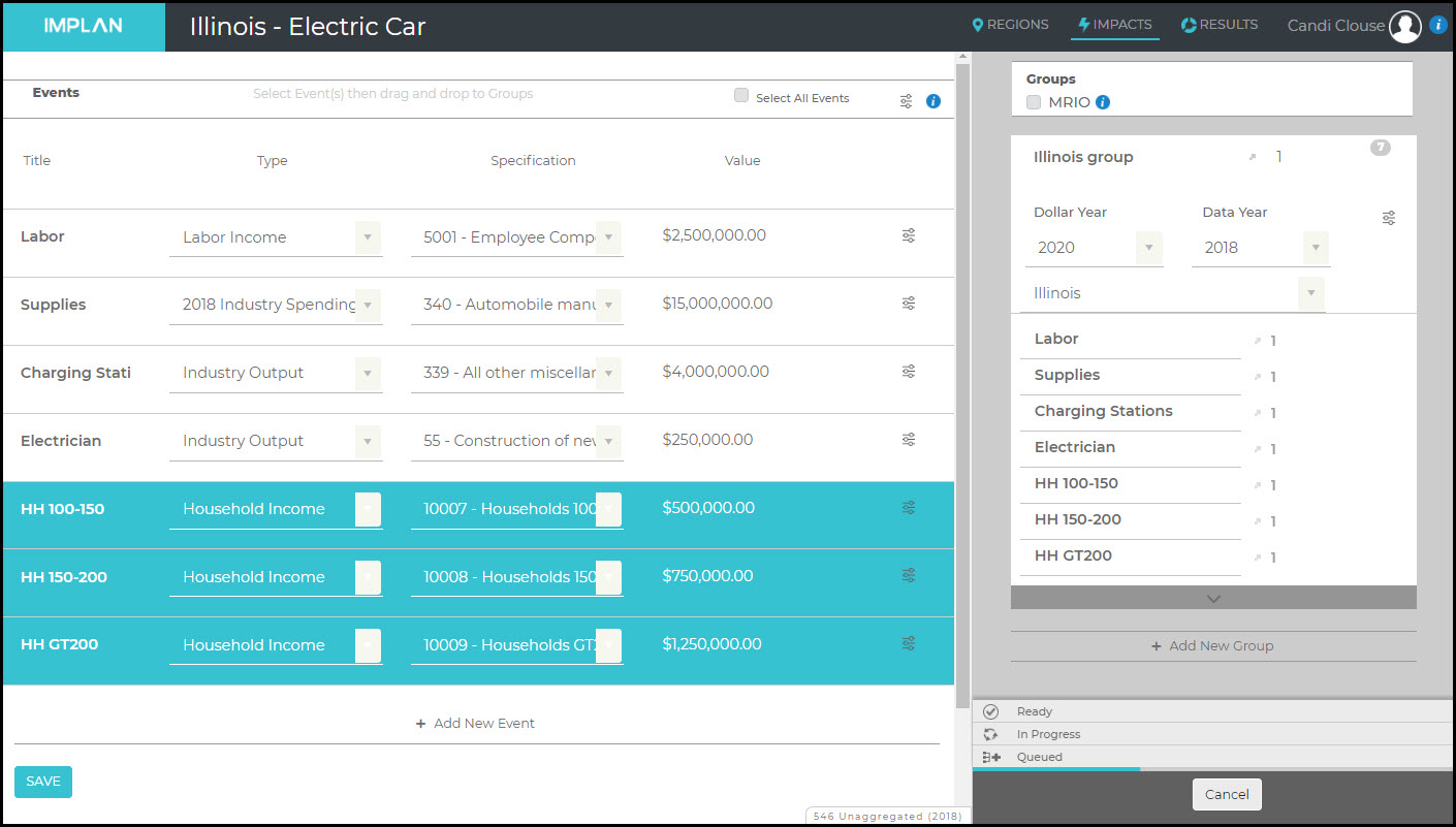
If we know that higher income Households will see significant savings, this can be modeled by a few Household Income Events. In this example, we are told that Households that earn between $100-150K will save $500K, Households that earn between $150-200K will save $750K, and Households that earn more than $200K will save $1.25K, we create one Event for each earning level.
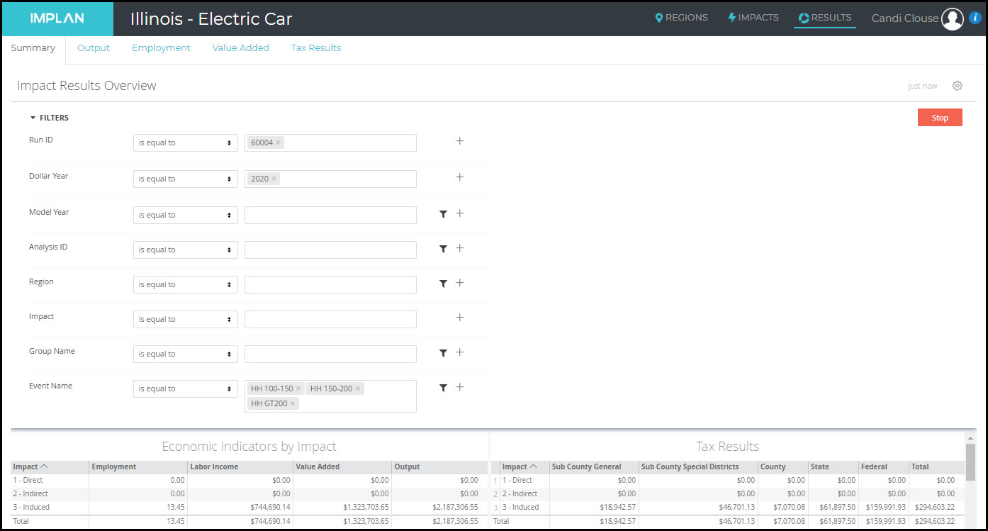
Again using the Filter on the Results screen, once these additional Events have been analyzed, and choosing only the three Household Events and clicking Run, we see the Results from the Household savings.
https://implan.com/wp-content/uploads/electric-vehicle-economic-impact.jpg14142121Joe Demskihttps://implan.com/wp-content/uploads/Market-site-Logo-resized-2-1.jpgJoe Demski2020-08-12 11:20:572025-02-06 15:52:42Electric Vehicles: Industry on the Move
IMPLAN now includes data for occupation employment, wage, and core competency (knowledge, skills, abilities, education, work experience, and on-the-job training levels for each occupation). This new data offering allows for expanding employment impact results to include occupation detail (with associated wage, education, and skill detail) in addition to Industry detail. These data are also applied to the IMPLAN study area data, providing important insights into a Region’s existing skill force, the skill requirements of various industries, and more.
This article describes the methods and sources the IMPLAN Data Team uses to estimate these occupation and core competency data.
DATA SOURCES
There are four main sources for the IMPLAN Occupation Data. The most recent data years for each are utilized.
Bureau of Labor Statistics (BLS) Occupational Employment Survey (OES)
Provides data on knowledge, skills, abilities, education, work experience, and on-the-job training by occupation.
A new database version is released whenever updates are made.
For all sources, IMPLAN uses the most recent data release as of the time the occupation data generation process begins.
Occupation Data Year
OES
BLS
PUMS Data
O*NET
2018
2018
2018
2018
24.2
OCCUPATION EMPLOYMENT & COMPENSATION
It is important to note that IMPLAN reports occupation data only for the Wage and Salary Employment component of Total Employment, and therefore only for the Employee Compensation component of Labor Income. Note that proprietors are excluded from occupation-related IMPLAN data. This maintains consistency with Occupational Employment Statistics (OES) coverage only of “employees.”
OES data on occupation employment and wages by industry generally are available on an annual basis. IMPLAN relies most heavily on this dataset for occupation employment and compensation. The raw OES data report employment and wages by BLS SOC code, which has a hierarchy similar to North American Industrial Classification System (NAICS) codes. The SOC hierarchy occurs in 4 levels: major, minor, broad, and detail. OES data sometimes omit a level in the SOC hierarchy, e.g., reporting positive values at the detail level and its broad parent level, but nothing at the corresponding parent minor level. OES data also contain suppressions due to non-disclosure rules, with the result that a broad level code with 10 employees might report only one child detail code with 7 employees, leaving no information about the occupations of the remaining 3 employees.
When estimating occupation employment by industry, IMPLAN estimates values where that value would be non-disclosed in the OES data and ensures consistency among levels. That is, if 2 detail codes contain 5 employees each, the corresponding broad code will have 10 employees. Sometimes this requires overwriting published values that are inconsistent with other published values while ensuring that the IMPLAN data maintain as much consistency with the raw data as possible. IMPLAN’s method of disclosing missing values entails using data from aggregations at a higher NAICS or SOC level, as well as controlling lower-level values to known higher-level aggregates. Wage values are treated similarly to employment values in the disclosure process.
IMPLAN matches the disclosed and consistent occupation by industry employment data to IMPLAN Industries. In some cases, OES does not provide any coverage of an industry, such as agriculture and private households. In this case, IMPLAN supplements the OES data with data from the BLS Employment Projections, which also provide data on occupation employment by industry, but not on occupation wages by industry. Wage data from OES are substituted in this case. IMPLAN uses other BLS data to estimate military occupation employment, and deviates from the SOC system for coding military occupations. Occasionally, OES provides detail only to a NAICS level that encompasses more than one IMPLAN Industry. In such cases, IMPLAN applies the distribution of occupation employment for that NAICS code to all constituent IMPLAN Industries. Additionally, there are cases in which IMPLAN refines initial occupation estimates for an IMPLAN Industry that uses occupation data for an aggregate NAICS by accounting for a sibling industry that uses occupation data for a more detailed level of the same aggregate NAICS.
IMPLAN uses the occupation hours data from PUMS to adjust its estimates of occupation wages. The OES data on wages by occupation assume that each occupation works 2,080 hours per year (40 hours * 52 weeks), except in some cases in which it provides only an hourly wage. If IMPLAN followed that assumption, it might attribute too much compensation to occupations that tend to work fewer than 2,080 hours per year. For example, consider a hypothetical restaurant industry that has only one business. That restaurant has one waiter position, which is hired all year long but only for 20 hours per week and is paid $10 per hour. The waiter position should not be assumed to earn $10 * 2,080 = $20,800 per year; rather, the waiter would earn $10 * 2,080 * (20 / 40) = $10,400 per year. If this business also employs a restaurant manager, who works 40 hours per week and earns $20 per hour, the manager earns a total of $41,600. Properly accounting for hours worked means that the manager earns 80% of the total compensation paid by the business and in the industry, with the waiter earning the remaining 20%. Failing to account for hours worked gives the manager 67% and the waiter 33%.
CORE COMPETENCIES
KNOWLEDGE, SKILLS, ABILITIES, EDUCATION, WORK EXPERIENCE AND ON-THE-JOB TRAINING
Developed by Philip Watson, Ph.D.
Each occupation in IMPLAN is deconstructed into their constituent Knowledge, Skill, and Ability (KSA) elements as well as education levels, work experience, and on-the-job training using Bureau of Labor Statistics (BLS) data and O*NET™ data. The KSAs along with education, experience, and training are referred to as the “core competencies.”
O*NET™ data report 33 unique knowledge elements, 35 unique skill elements, 52 unique ability elements, 12 unique educational attainment elements, 11 unique work experience levels, and 9 unique on-the-job training levels. Descriptions of these core competency elements can be found in the Core Competencies spreadsheet.
In order to generate workforce reports, IMPLAN occupation data must be bridged to the core competencies. However, neither O*NET™ databases nor the BLS provides a bridge between occupations and core competencies; rather, they report values on two scales for each occupation and KSA combination. The scales that are reported are a 0-5 measure of “importance” and a 0-7 measure of “level.” Combining these two scales into a bridge of occupation employment to measures of KSA endowments requires some assumptions and empirical calculations. The assumptions used, while not intended to be regarded as the only set of assumptions that could be used to generate the bridges, were empirically tested to ensure that the resulting bridges accurately predicted occupation wages and presented a reasonable measure of the KSAs associated with each occupation.
ASSUMPTIONS
The first assumption used in generating the bridges is that the two KSA scales would be combined using a multiplicative interaction between the scales. The use of a multiplicative relationship rather than an additive interaction deemphasizes very small values for either the level or the importance and creates a higher weight for KSA elements that have higher values for both the level and the importance. Alternative interactions were also explored, including additive, arithmetic means, and geometric means, but the multiplicative interaction was found to be the best across multiple empirical tests.
The second assumption is that core competency endowments are associated with the occupations to which people are employed (or potentially unemployed) in a region rather than directly to the people themselves. Therefore when a person moves from one job to another within a region, the core competencies in the region change even though the same people reside and work there as before. More technically, the core competencies generated here are a measure of the expected human capital endowments in the region given the current occupation mix of employment in the region. This assumption relates directly to the third assumption below.
The third assumption in generating the bridge is that every occupation uses the same absolute amount of KSAs and, therefore, the differences between the KSAs associated with different occupations are in their distribution, not their level. This assumption is useful due to the incompatible units across KSA elements. The result of this assumption is that every occupation can be thought of as using 100 units of knowledge elements, 100 units of skill elements, and 100 units of ability elements in varying distributions. When a worker moves from one job to another, the worker’s mix of KSAs change, but the overall amount of total KSAs which the worker possess does not change. Likewise, under this assumption education and training do not necessarily increase the absolute level of KSAs in a region; rather, they simply enable people to move from one occupation to a different occupation with a different (and presumably more valuable) set of associated KSAs.
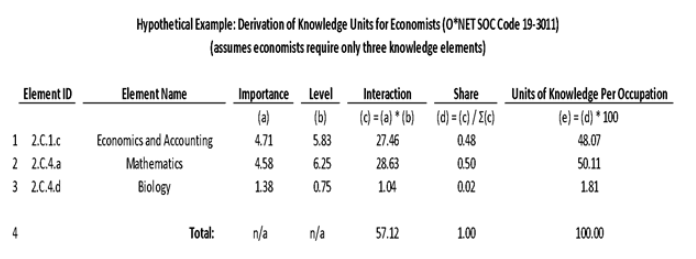
The chart below presents a numerical example of calculating units of knowledge elements from the O*NET data. The example is simplified, as O*NET includes many more knowledge elements for the economist occupation. According to this example, if an economy contains only one job, and that one job is held by an economist, the economy would have 100 units of knowledge, allocated among the three types listed below. The calculation is the same for other occupations and for other KSA types.
The other core competencies outside of the KSAs were more straightforward in their bridging to occupation data. Education, work experience, and on-the-job-training data from the O*NET™ database are reported as proportions of persons employed in a given occupation that each have a given level of education or training, respectively. O*NET™ data report 12 levels of educational attainment, 11 levels of work experience, and 9 on-the-job-training categories. Since they are already reported as proportions, the bridge to IMPLAN occupation data is direct and does not require any additional assumptions. The education, work experience, and training categories can also be found in the Core Competencies spreadsheet. However, similar to the KSAs, the education and training elements are occupation-based and not individual-based; therefore, they are not to be thought of as the direct endowments of the individuals in a region, but rather as the expected endowments relative to the occupation employment in the region.
While O*NET data covers the majority of OES occupations, there are occupations in the O*NET database that lack data. For example, the “all other” occupations (SOCs ending in 9: xx-xxx9) often lack O*NET data. In such cases, core competency data for the occupation is estimated using the core competency estimates of sibling level occupations weighted by each competency’s survey response size as provided by O*NET. This approach assumes that the “all other” occupation reflects the competency emphasis of the sibling occupations. Additionally, military occupations were estimated using similar means in order to bridge O*NET data to IMPLAN’s custom military occupation codes.
Given the data and assumptions described above, IMPLAN can estimate endowments of the respective core competencies which will sum to 100 times the same total as the occupation employment total in the region. For example, if there are 1,000 occupation jobs in a given region, then there will be 1,000*100 occupation equivalents of knowledge, 1,000*100 occupation equivalents of skills, and 1,000*100 occupation equivalents of abilities. These occupation equivalents will vary widely by region based on the industrial and occupation employment mix in the respective region.
The IMPLAN Development Team works tirelessly to ensure that your experience using the application is as smooth as possible. Once in a while, however, you will see “Oops! Something went wrong” or the dreaded coral colored error bar shows up on your screen.
The first thing we recommend to fix any issues is to clear your cache and then logout and log back into your account. If that doesn’t work, here’s what all of these error messages mean and how to fix them.
WEB BROWSER
IMPLAN recommends using Google Chrome to get the best experience. IMPLAN also works in Edge, Firefox, and Safari. Internet Explorer is no longer supported.
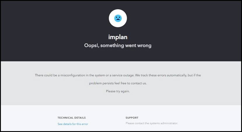
OOPS SOMETHING WENT WRONG
It’s never good when a frowny face shows up on your screen. The error notes “There could be a misconfiguration in the system or a service outage. We track these errors automatically, but if the problem persists feel free to contact us. Please try again.”
Cause
Solution
Using Internet Explorer
Literally use anything else
Using an outdated bookmark to login
Go straight to app.implan.com to login
Outage or server disruption
Our Product Team has automatically been alerted and will be working on this fix ASAP
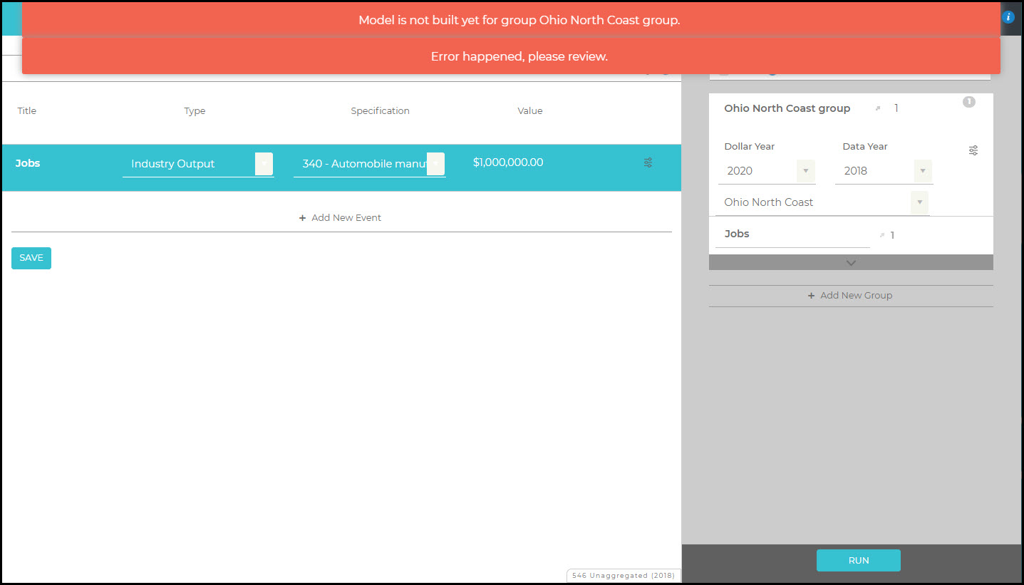
CORAL ERROR BAR
Sometimes you will see a coral error bar pop up on your screen. Here are the reasons why the error is being triggered.
Cause
Solution
Specification Code cannot be negative or zero.
Choose an appropriate selection in the Specification field and hit Run.
Model is not built yet for group X.
IMPLAN is building your Combined Region or Custom Aggregation Scheme; give it a few minutes and try again. You can check to see if a Region is done building by checking for the information icon being available on the Regions screen.
Object Progress Event
Take out any special characters you have in your name like #, +, %, etc.
This action cannot be completed because one or more Groups has no name. Please name all Groups.
One or more of your Groups on the right side of the screen is missing a name, please add one.
Please ensure that all groups have Region selected from the Regions drop down menu for each group
Ensure that there is a Region name populated in each Group
BLANK SCREEN
If you navigate to a screen in IMPLAN and you don’t see the tables you expect, refresh your screen. If that doesn’t work, clear your cache and then logout and log back into your account.
IF ALL ELSE FAILS
Your Customer Success Manager is here to help! Shoot an email to support@implan.com and one of our team members will look into the problem to ensure you can successfully complete your project.
https://implan.com/wp-content/uploads/Market-site-Logo-resized-2-1.jpg00Joe Demskihttps://implan.com/wp-content/uploads/Market-site-Logo-resized-2-1.jpgJoe Demski2020-08-12 11:18:162020-08-12 11:18:16Error Messages & How to Fix Them
There are three possible types of Effects included in the Results of each analysis performed in IMPLAN: Direct, Indirect, and Induced. Direct Effects are the initial Final Demand Effect. Indirect Effects are generated due to demands from the regional supply chain to produce the final goods & services in the analysis, while Induced Effects are generated due to demands from households whose income is earned directly or indirectly due to their job activity in production being analyzed.
EFFECTS BY EVENT TYPE
Events that are designed to analyze Final Demand including Industry Events (Output, Employment, Employee Compensation and Proprietor Income), Industry Contribution Events, Commodity Output Events, and Institutional Spending Pattern Events. These will each have a Direct, Indirect, and Induced Effect. As shown in the table below this is not the case with all Event Types.
Direct, Indirect, & Induced
Indirect & Induced Only
Induced Only
Industry Events
Industry Spending Pattern Events
Labor Income Events
Industry Contribution Events
Household Income Events
Commodity Output Events
Institutional Spending Pattern Events
Industry Spending Pattern Events are designed to analyze effects due to the regional supply chain of the specified Industry. Industry Spending Patterns are made up of the Intermediate Inputs for the Industry and produce only Indirect and Induced Effects. Labor Income and Household Income Events are only designed to capture effects due to income earned in the analysis, producing Induced Effects only. Because Industry Spending Patterns Events and the two Income Events do not specify the exogenous change in Final Demand, these Event Types will not have a Direct Effect.
These categorization of Effects by Event Type are by design in IMPLAN and cannot be adjusted internally in the IMPLAN application. That being said, there are cases where it is appropriate to add in the “missing” Direct Effect or recategorizing Effects in the Results produced in IMPLAN.
DOWNLOAD RESULTS IN EXCEL
If manipulation of your Results is appropriate, start by downloading the results in the Results screen for whichever table you’d like to report. According to the following scenarios, adjust your Results accordingly. Remember to make the corresponding changes made in the Summary Results to any other Results tables you’ll be reporting.
RECATEGORIZING EFFECTS
ANALYSIS-BY-PARTS: INDUSTRY SPENDING PATTERN
Analyzing an Industry using Analysis-by-Parts is a workaround for the customization limitations in a single Industry Event. For this reason, the Results are not as straightforward as the Results produced in an Industry Event. When using an Industry Spending Pattern in your ABP, there will be only Indirect and Induced Effects. According to the IMPLAN Results, there is no Direct Effect, but adding in the known Direct Effect can be important for communicating the Total Effects of your analysis. If you’ve completed an ABP, you already have information on the Direct Labor Income, which should be included in the calculation of Direct Value Added and Direct Output. For an ABP you also must know either Direct Output or Direct Intermediate Inputs. Remember how Output breaks down:
If not all the Direct factors are known, estimates of these factors can be made from the underlying Study Area Data using the information found in:
You will find Output value ratios for the Industry you want to use. If the Industry does not exist in the Region, the Proxy region information must be used. Employment can be estimated using the Output per Worker ratios that are provided in:
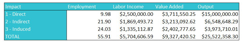
The Direct Effect you produce should replace the effects of all zeros in the downloaded Excel format Results. The existing Indirect and Induced Effects are correct as is. The added Direct Effects can be summed with the existing Indirect and Induced Effects by column to produce the accurate Total Effects.
ANALYSIS-BY-PARTS: BILL OF GOODS APPROACH
When applying the Analysis-by-Parts technique using the Bill of Goods (BOG) Approach you are using a series of Commodity and/or Industry Effects instead of an Industry Spending Pattern. In the Results, your Direct Effects are from the Commodity/Industry Events, which actually reflect the Intermediate Input purchases made by the true Direct business. The Results should be modified such that these Direct Effects are reclassified as Indirect Effects. Once this step is completed, you should have only Indirect and Induced Effects, similar to the results when using an Industry Spending Pattern in an ABP as shown above. You can then add in the true Direct Effect as described in the previous section. Don’t forget to sum a new Total Effect.
Remember, if you’ve completed an ABP, you already have information on the Direct Labor Income, which should be included in the calculation of Direct Value Added and Direct Output. In this ABP approach, you also have information on the Direct Intermediate Inputs, which were analyzed as Commodity Events. If you’ve analyzed Commodity Output values that equal the total spending on each Commodity (locally and non-locally) by the Direct business, then the sum of Commodity Output values in all Commodity Output Events is equal to Direct Intermediate Inputs and can be summed with Direct Value Added to produce Direct Output.
If you are using this analysis approach because the Industry you are analyzing is not an Industry in the IMPLAN Industry Scheme and you are missing information about the Direct Effect, we recommend basing the Direct Effect calculations on the Industry that is most similar to the Industry you are analyzing with the BOG Approach.
INTERNALIZING OTHER INSTITUTIONAL EFFECTS
When analyzing Events in a single Region in IMPLAN, the application will generate effects due to spending by only one Institution: Households (in a Multi-Regional analysis trade “spending” is also internalized). Revenue for other Institutions can also be affected. For example, the Tax tab of your Results displays all the fiscal revenue supported by your analysis, but there will be no Direct, Indirect, or Induced Effects due the estimated tax collection being spent by the different levels of government.
Additional Events can be analyzed to produce these effects if enough information is known on how the Institution’s spending will be affected. In any analysis that includes Institution spending of revenue derived from an already present Direct Effect, you should treat all effects of that spending as Induced. Direct, Indirect, and Induced Effects should be summed and recategorized as Induced Effects when using an Institutional Spending Pattern or any other Event Type to manually internalize the effects of secondary demands from Insitutitions (other than Households) expected to be supported by the other Events being analyzed.
These Induced Institutional Effects can be combined with the original Effects produced by the Event. In which case a new Total Effect would need to be calculated.
https://implan.com/wp-content/uploads/Market-site-Logo-resized-2-1.jpg00Joe Demskihttps://implan.com/wp-content/uploads/Market-site-Logo-resized-2-1.jpgJoe Demski2020-08-12 11:17:262020-08-12 11:17:26Categorizing Effects: Adding Back the Direct & Including Institutional Spending
Public transit in the form of buses and rail lines are essential to functioning cities. Governments make huge investments in infrastructure ensuring access for all residents. This article looks at how these investments look in IMPLAN.
OPERATIONS
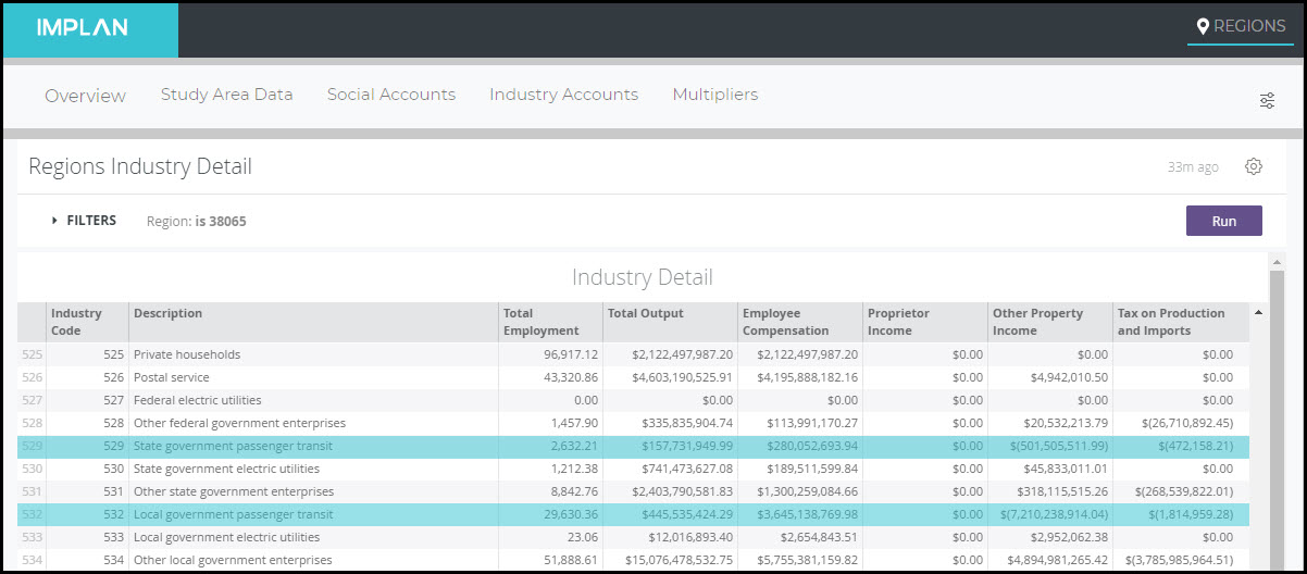
Public transit comes in the form of two Industries in IMPLAN: 529 – State government passenger transit and 532 – Local government passenger transit. Both of these Industries are government-based and operate by selling goods and services to the public. Generally, they operate like private sector firms; they hire employees and purchase Intermediate Inputs. Other government transportation related spending and investments are captured in IMPLAN within two Institution categories: 12001 – State/Local Government Other Services and 12004 State/Local Government Investment.
Below shows the two public transit Industries for New York in 2018. Note not all areas will have both local and state run transit.
The first thing to notice is that both of these Industries have no Proprietor Income. They also both have negative OPI and TOPI. Negative OPI indicates that the Industry spent more than it brought in as revenue – it ran a deficit. Negative TOPI is due to the given Industry receiving subsidies from the government.
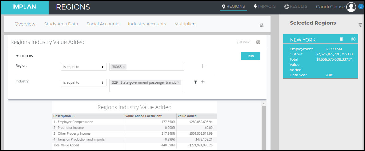
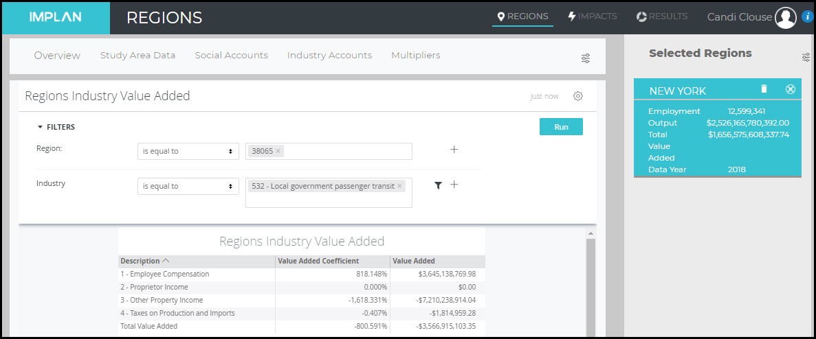
To model an expansion of spending on transit, an Industry Event with the appropriate values is best. To examine how transit contributes to the regional economy as it is funded currently, an Industry Contribution Analysis is best. Note that when any type of analysis is run on one of these Industries (in the New York 2018 Region and many others), the Results will show no Direct Proprietor Income, negative TOPI, and negative OPI. In fact, in the case of this Region, the Negative TOPI and OPI are so significant, the net Value Added for these Industries are negative. This will result in a negative Direct Value Added when these Industries are analyzed. Shown below for the Region of NY 2018, the Value Added Coefficient for the State government passenger transit Industry is about -141%, and -801% for the Local government passenger transit Industry.
The construction of new transit lines falls under IMPLAN Industry 56 – Construction of other new nonresidential structures. When analyzing any construction, the value entered in Industry Output should be the full cost of the structure, and only the structure, including hard costs and soft costs. For further details, visit the article Construction: Building the Analysis.
Capital purchases can be a bit tricky and need to be analyzed separately from construction costs. Perhaps your local authority is purchasing light rail cars or hydrogen fuel cell buses. In today’s global economy, it is unlikely that these are produced within your Region, so the entirety of the cost would be considered a leakage. If the capital purchases are made in your Region, it is typically appropriate to choose the manufacturing Industry that produced the item when analyzing the purchase via an Industry Output Event. For example, if a locally made bus is purchased, choose Industry 343 – Motor vehicle body manufacturing, and enter the cost of the bus. For more information on capital purchases, check out the article Analyzing Capital Investments.
https://implan.com/wp-content/uploads/Market-site-Logo-resized-2-1.jpg00Joe Demskihttps://implan.com/wp-content/uploads/Market-site-Logo-resized-2-1.jpgJoe Demski2020-08-12 11:12:192020-08-12 11:12:19All Aboard! Modeling Public Transit
Did you ever wonder how much local bread your local supermarkets buy? Or how much local auto manufacturers spend on local tires? The process to find this answer may seem complicated, but it is actually relatively simple. Here’s how.
THE PROCESS
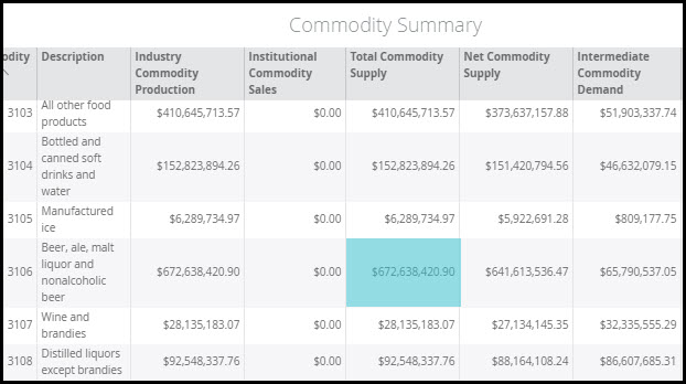
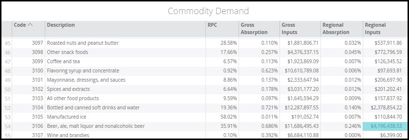
Let’s examine how much local beer is purchased by local restaurants in Greater Milwaukee. Start by selecting your Region (Milwaukee-Waukesha, WI MSA 2018 shown below) and heading into the data for Commodity 3106 – Beer, ale, malt liquor and nonalcoholic beer.
The Total Commodity Supply for beer is $672,638,420.90. This represents the total beer supply produced in Milwaukee by both Industries and Institutions.
> Filter for Industry 509 – Full-service restaurants
> Regional Inputs
Scroll to Commodity 3106 – Beer, ale, malt liquor and nonalcoholic beer and find the value for Regional Inputs. For the Milwaukee-Waukesha, WI MSA this is $4,196,438.53. Regional Inputs show the amount that restaurants spend locally on beer during the Data Year. Note that the Gross Inputs of $11,686,495.43 represent the total annual spending on beer by full-service restaurants. We then know that local restaurants are spending 35.91% of their beer budget on local brews (RPC = 35.91%).
STEP 3: DIVIDE THE RESULTS
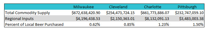
The Regional Inputs of $4M divided by the Total Commodity Supply of $673M tell us that Milwaukee restaurants are buying less than 1% of total local beer production. Given how much beer production occurs in the Region, the percentage of local beer production that is purchased by local restaurants is quite low. The table below compares four cities on the percentage that local restaurants spend on local beer.
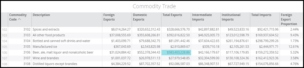
Now we can look at exports. Foreign Exports tells us the total local production that is exported outside the U.S. The Domestic Exports tells us the total local production that leaves Greater Milwaukee but stays in the U.S. The Total Exports is a combination of these two. The Total Exports from Milwaukee is $583,403,228.86. Taking this divided by the Total Commodity Supply of $672,638,420.90 tells us that 87% of the locally produced beer is exported from the MSA. Therefore, 13% stays local – which is known as the Average RSC (Regional Supply Coefficient).
STEP 5: INCREASE LOCAL BEER PURCHASES
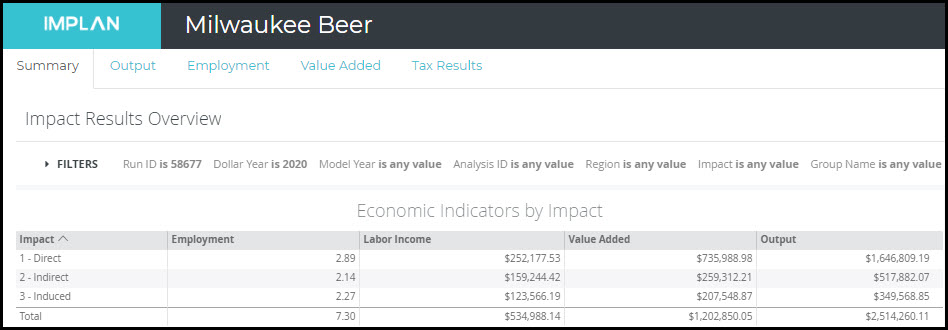
Let’s say local restaurants want to commit to purchasing a full 50% of their beer from local breweries. They are currently spending a total of $11,686,495.43 on beer, so half would be $5,843,247.72. They are currently spending $4,196,438.53, so they would need to increase their local buy by $1,646,809.19. We can run this as an Industry Output Event.
The Results show us that the increase in $1,646,809.19 in local breweries supports a total Output of $2,514,260.11; a multiplier of 1.53. This will support almost 3 employees at the brewery and 4 additional employees in the Indirect and Induced Effects; a multiplier of 2.53.
IMPLAN introduces new data each year. With new data, comes new multipliers. In general, it is not advisable to treat annual IMPLAN datasets as a time series as our data sources and methods often change from year to year. Additionally, some of our raw data sources revise estimates, so that, for example, what a source reports about 2013 in 2018 is different from that source would report about 2013 in 2019. This is especially true of data from the Bureau of Economic Analysis. On a 5-year basis (following the incorporation of a new BEA Benchmark, Census of Agriculture, and IMPLAN Industry scheme) we publish Panel Data, spanning from 2001 to the latest annual IMPLAN data year, to facilitate year-over-year analysis. These datasets use all the data and methodological changes incorporated over the preceding 5 years, and are reported in the same (latest) IMPLAN sectoring scheme.
DETERMINING MULTIPLIER SIZE
Again, as the data changes over time, it is not uncommon to see changes in the multipliers. Changes of less than 10% (positive or negative) are quite routine and expected. Larger changes can be expected if comparing non-consecutive years or years that span one of our 5-year data sets (see next section on Five Year Data). Employment and Value Added multipliers can vary greatly across geographies and years whereas Output multipliers tend to be relatively more stable.
Multipliers are influenced by many factors, so it is not possible to isolate a single factor when examining their changes over time. These factors include some that are specific to the geography in question, while others are specific to the Industry in question. Still others may be related to global trends. Here are some reasons why there are yearly changes.
A greater reliance on imports (whether foreign or domestic) will result in lower RPCs in general, which, all else equal, reduce multipliers.
When productivity, as defined as Output per worker, rises in a given Industry, the Employment per dollar of Output falls. All else equal, a smaller Direct Employment will result in a larger Employment multiplier for this Industry.
Change in Labor Income per dollar of Output, whether from changes in wage rates or the changing fortunes of proprietors, will change the magnitude of Induced Effects, and therefore multipliers. Proprietor Income can be negative and can vary substantially from one year to the next.
A decrease in a multiplier can also be caused by a large increase in corporate profits and/or taxes paid per dollar of Output. Corporate profits make up the bulk of Other Property Income (OPI), a component of Output that is treated as a leakage in I-O modeling, in the sense that they are not spent within the model and therefore do not generate Indirect or Induced Effects. Similarly, all taxes, while accounted for in the tax impacts report, do not generate additional rounds of impacts. The larger the percentage of Output that goes to OPI and taxes, the less leftover to drive Indirect and Induced Effects.
FIVE YEAR DATA
Some raw data sets are released only every 5 years; thus, larger year-over-year changes can be expected when comparing IMPLAN data across two years that span the release of one of these 5-year data sets, like between 2017 (536 Industry Scheme) and 2018 (546 Industry Scheme).
THE BEA BENCHMARK I-O TABLES – RELEASED EVERY 5 YEARS
A new BEA Benchmark provides new industry spending patterns for all IMPLAN industries. The magnitude of total Intermediate Input purchases per dollar of Output and the relative mix of input purchases both influence Indirect Impacts, and the Induced Impacts associated with those Indirect Impacts.
A new BEA Benchmark also provides data on the foreign imports and exports of Commodities. While we have annual Census data for the foreign trade of all shippable Commodities, no such data source exists at this level of Commodity detail for the annual foreign trade of services. Thus, we turn to the BEA Benchmark to give commodity detail to the NIPA control total for the foreign trade of services.
A new BEA benchmark also provides new national indicators of the relationship between Output, Employee Compensation, gross operating surplus (PI + OPI), and TOPI. These relationships are especially important for farm data, as many of our annual sources report data for agriculture only at the farm level. We use the BEA Benchmark for other components, including detailed Commodity margins, which will have more minor effects on multipliers.
THE CENSUS OF AGRICULTURE – RELEASED EVERY 5 YEARS
The Census of Agriculture provides us with data on farm counts (both proprietor-owned and corporate-owned) by farm sector, by county. These data are used annually to distribute state-level farm Output data to counties and to provide Industry detail to the aggregate farm BEA REA data we use for farm Industry Employment and Labor Income.
INVESTIGATING A CHANGE
If you see a change in multipliers that has you curious, here are four steps to investigate what may be causing it.
STEP 1: PRELIMINARY CHECKS
Are both data sets in the same Industry Scheme?
Is any aggregating or splitting needed to make the Industries comparable?
STEP 2: EXAMINE THE STUDY AREA DATA
Has Employment per Output changed significantly?
Has Labor Income per Output changed significantly?
STEP 3: EXAMINE SPENDING PATTERN AND RPCS OF TOP ITEMS
Has the ratio of Intermediate Inputs per Output changed significantly?
Have the RPCs of the top few Commodities purchased by the Industry changed significantly?
STEP 4: CONTACT IMPLAN SUPPORT FOR ASSISTANCE
Help us help you! To expedite the process of investigating a value, it is extremely helpful for us to have the following details at the outset:
What type of multiplier are you concerned with (Employment, Output, etc.)?
What specific IMPLAN Industry or Industries, with the associated Industry number(s) are in question?
What are the two data years being compared?
What is the geography in question?
Is the multiplier in question from the Multipliers Report in IMPLAN or calculated based on impact results?
Then shoot an email to support@implan.com and our Data Team will take a look!
https://implan.com/wp-content/uploads/Market-site-Logo-resized-2-1.jpg00Joe Demskihttps://implan.com/wp-content/uploads/Market-site-Logo-resized-2-1.jpgJoe Demski2020-08-12 11:10:172020-08-12 11:10:17Multipliers Changing Over Time
Multipliers measure the economic change within a Region that stems from economic activity from a change in Final Demand. They are a measure of an Industry’s connection to the wider local economy by way of input purchases, payments of wages and taxes, and other transactions. They are the total production impact within the Region for every unit of direct production.
There are two main types of multipliers. For more details, check out the article Understanding Multipliers.
Type I Multiplier = (Direct Effect + Indirect Effect) / (Direct Effect)
Type SAM Multiplier = (Direct Effect + Indirect Effect + Induced Effect) / (Direct Effect)
And yes, sometimes they are negative. Here are the details.
DETAILS
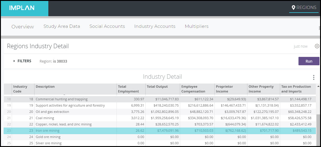
Let’s take a look at an example. In Alabama 2018 Industry 23 – Iron Ore Mining, there is negative Proprietor Income.
So we know that there was a net loss for Proprietor Income in 2018 in this Industry. Proprietors could have lost money or spent more money from savings than they earned. This doesn’t mean that they went out of business. They could be just using savings or borrowing money to maintain their cash flow. For further details on why this happened, read the article The Curious Case of the Negative Tax: Agriculture Subsidies, Profit Losses, and Government Assistance Programs.
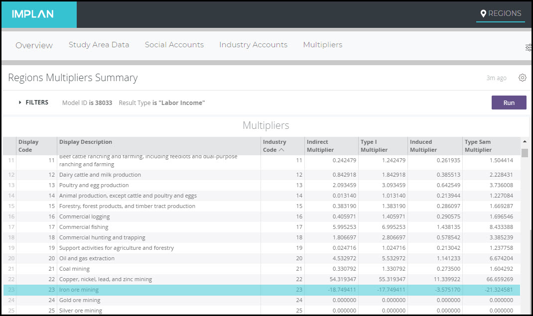
Labor Income is equal to Proprietor Income + Employee Compensation. Because we saw a negative in Proprietor Income that was larger than the positive Employee Compensation, there is negative Labor Income in this Industry. When we analyze increased production in this industry, IMPLAN estimates negative Direct Labor Income. When an Industry has this negative relationship between Output and Labor Income, the total Labor Income supported by increased production is typically positive while the Direct Labor Income is negative. This produces a negative Labor Income Multiplier.
In a bad year (low prices or spikes in operational costs), an Industry can lose money. Losses in any piece of Value Added (Employee Compensation, Proprietor Income, Taxes on Production & Imports, or Other Property Income) can create a negative multiplier if those losses aren’t offset by larger gains in another piece of Value Added. For example, in IMPLAN, the combination of Proprietor Income and Other Property Income equals operating surplus. The operating surplus of an Industry is simply its profits – that is, value of production minus all operational expenditures. If the negative operating surplus exceeds Employee Compensation plus Taxes on Production & Imports, then total Value Added will be negative. Industries with a negative relationship between Output and Value Added usually have a negative Value Added Multiplier, like in the case of Labor Income.
The data Behind the “i” is helpful for better understanding the Results produced in your analysis.
CALCULATION STEPS:
To calculate the leakages due to spending on Intermediate Inputs outside of the Study Region click on the “i” icon next to the Selected Region and navigate to:
Social Accounts
> Balance Sheets
> Industry Balance Sheet
> Commodity Demand
In the Commodity Demand table, you’ll find the following columns (be sure to filter by your Industry of interest):
Gross Absorption = the proportion of Total Industry Output for this industry that goes toward purchases of each commodity. Gross Absorption is calculated as Gross Inputs/Total Industry Output. Total Gross Absorptions will be less than one, with the remainder of Total Industry Output going toward Value-Added.
Regional Absorption = the proportion of Total Industry Output for this industry that goes toward local purchases of each commodity. Regional Absorption can be calculated as Gross Absorption * RPC
Therefore, Total Gross Absorption – Total Regional Absorption = percentage of Total Industry Output that is spent on Intermediate Inputs outside of the Region. This percentage multiplied by Total Industry Output are the Intermediate Input dollars leaked out from the Direct Effect.
Take for example “Industry 56 – Construction of other new nonresidential structures” in Pennsylvania 2018. The Total Gross Absorption is 52.057% and the Total Regional Absorption is 31.671%. This means about 52% of Output is allocated to Intermediate Inputs overall, and about 32% of Output is allocated to Intermediate Inputs in the Region. Therefore, about 20% of Output is allocated to Intermediate Inputs outside of the Region.
% of Total Industry Output spent on non-local Intermediate Inputs = 52.057% – 31.671% = 20.386%
When analyzing $1M of new Output in this Industry in PA, IMPLAN would estimate $203,860 of the $1M of new production as being spent on non-local Intermediate Inputs. The remaining $796,140 includes local Intermediate Inputs ($316,710) and Value Added ($479,430).
https://implan.com/wp-content/uploads/Market-site-Logo-resized-2-1.jpg00Joe Demskihttps://implan.com/wp-content/uploads/Market-site-Logo-resized-2-1.jpgJoe Demski2020-08-12 11:08:092020-08-12 11:08:09Calculating Leakages of Direct Intermediate Inputs